Last time on FAIC we reviewed the meaning of “expected value”: when you get a whole bunch of samples from a distribution, and a function on those samples, what is the average value of the function’s value as the number of samples gets large?

I gave a naive implementation:

public static double ExpectedValue<T>(
    this IDistribution<T> d,
    Func<T, double> f) =>
  d.Samples().Take(1000).Select(f).Average();

public static double ExpectedValue(
    this IDistribution<double> d) =>
  d.ExpectedValue(x=>x);

Though short and sweet, this implementation has some problems; the most obvious one is that hard-coded 1000 in there; where did it come from? Nowhere in particular, that’s where.

It seems highly likely that this is either too big, and we can compute a good estimate in fewer samples, or that it is too small, and we’re missing some important values.

Let’s explore a scenario where the number of samples is too small. The scenario will be contrived, but not entirely unrealistic.

Let’s suppose we have an investment strategy; we invest a certain amount of money with this strategy, and when the strategy is complete, we have either more or less money than we started with. To simplify things, let’s say that the “outcome” of this strategy is just a number between 0.0 and 1.0; 0.0 indicates that the strategy has completely failed, resulting in a loss, and 1.0 indicates that the strategy has completely succeeded, resulting in the maximum possible return.

Before we go on, I want to talk a bit about that “resulting in a loss” part. If you’re a normal, sensible investor like me and you have $100 to invest, you buy a stock or a mutual fund for $100 because you believe it will increase in value. If it goes up to $110 you sell it and pocket the $10 profit. If it goes down to $90, you sell it and take the $10 loss. But in no case do you ever lose more than the $100 you invested. (Though of course you do pay fees on each trade whether it goes up or down; let’s suppose those are negligible.) Our goal is to get that 10% return on investment.

Now consider the following much riskier strategy for spending $100 to speculate in the market: suppose there is a stock currently at $100 which we believe will go down, not up. We borrow a hundred shares from someone willing to lend them to us, and sell them for $10000. We pay the lender $100 interest for their trouble. Now if the stock goes down to $90, we buy the hundred shares back for $9000, return them to the owner, and we’ve spent $100 but received $1000; we’ve made a 900% return on the $100 we “invested”. This is a “short sale”, and as you can see, you get a 900% return instead of a 10% return.

(I say “invested” in scare quotes because this isn’t really investing; it’s speculation. Which is a genteel word for “gambling”.)

But perhaps you also see the danger here. Suppose the stock goes down but only to $99.50. We buy back the shares for $9950, and we’ve only gained $50 on the trade, so we’ve lost half of our $100; in the “long” strategy, we would only have lost fifty cents; your losses can easily be bigger with the short strategy than with the long strategy.

But worse, what if the stock goes up to $110. We have to buy back those shares for $11000, so we’ve “invested” $100 and gotten a “return” of -$1000, for a total loss of $1100 on a $100 investment. In a short sale if things go catastrophically wrong you can end up losing more than your original investment. A lot more!

As I often say, foreshadowing is the sign of a quality blog; let’s continue with our example.

We have a process that produces values from 0.0 to 1.0 that indicates the “success level” of the strategy. What is the distribution of success level? Let’s suppose it’s a straightforward bell-shaped curve with the mean on the “success” side:

This is a PDF, and extra bonus, it is normalized: the total area under the curve is 1.0. The vast majority of the time — 99.9% — our investment strategy produces an outcome between 0.48 and 1.0, so that’s the area of the graph I’m going to focus on.

Aside: I know it looks a little weird seeing a bell-shaped curve that just cuts off abruptly at 1.0, but let’s not stress about it. Again, this is a contrived example, and we’ll see why it is irrelevant later.

Now, I don’t intend to imply that the “success level” is the return: I’m not saying that most of the time we get a 75% return. Let’s suppose that we’ve worked out a function that translates “strategy outcome level” to the percentage gain on our investment. That is, if the function is 0.0, we’ve not gained anything but we’ve not lost anything either. If it is 0.5 then our profits are 50% of our investment; if it’s -0.25 then we’ve taken a net loss of 25% of our investment, and so on.

Let’s propose such a function, and zoom in on the right side of the diagram where the 99.9% of cases are found: from 0.46 to 1.0. Here’s our function:

If our process produces an outcome of 0.54 or larger, we make between a 0% and an 18% return, which seems pretty good; after all the vast majority of the bulk of the distribution is to the right of 0.54. Now, in the unlikely case where we get an outcome from 0.48 to 0.54, we lose money; on the left hand end, we’re losing almost 200%; that is, if we put in $100 we not only fail to make it back, we end up owing $100.

The question at hand, of course, is what is the average value of the “profit function” given the distribution of outcomes? That is, if we ran this strategy a thousand times, on average what return would we get?

Well, we already wrote the code, so let’s run it: (Code can be found here.)

var p = Normal.Distribution(0.75, 0.09);
double f(double x) =>
  Atan(1000 * (x – .45)) * 20 – 31.2;
Console.WriteLine($”{p.ExpectedValue(f):0.##}“);

Aside: I’m ignoring the fact that if we get a sample out of the normal distribution that is greater than 1.0 or less than 0.0 we do not discard it. The region to the left of 0.0 is absurdly unlikely, and the region to the right of 1.0 has low probability and the value of the profit function is very flat. Writing a lot of fiddly code to correct for this problem would not change the estimated expected value much and would be a distraction from the far deeper problem we’re about to discover.

Also, I’m limiting the distribution to a support of 0.0 to 1.0 for pedagogical reasons; as we’ll see in later episodes, we will eventually remove this restriction, so let’s just ignore it now.

We get the answer:

0.14

Super, we will get on average a 14% return on our investment with this strategy. Seems like a good investment; though we have a small chance of losing big, the much larger chance of getting a solid 0% to 18% return outweighs it. On average.

Aside: It is important to realize that this 14% figure does not necessarily imply that typically we get a 14% return when we run this strategy, any more than the expected value of 3.5 implies that we’ll typically get 3.5 when we roll a d6. The expected value only tells you what the average behaviour is; it doesn’t tell you, for example, what the probability is that you’ll lose everything. It tells you that if you ran this strategy a million times, on average you’d get a 14% return, and that’s all it tells you. Be careful when making decisions relying upon expected values!

This 14% expected result totally makes sense, right? We know most of the time the result will be between 0% and 18%, so 14% seems like a totally reasonable expected value.

As one of my managers at Microsoft used to say: would you bet your car on it?

Let’s just run the code again to be sure.

0.14

Whew. That’s a relief.

You know what they say: doing the same thing twice and expecting different results is the definition of practicing the piano, but I’m still not satisfied. Let’s run it another hundred times:

0.14, 0.08, 0.09, 0.14, 0.08, 0.14, 0.14, 0.07, 0.07, 0.14, ...

Oh dear me.

The expected return of our strategy is usually 14%; why it is sometimes half that? Yes, there is randomness in our algorithm, but surely it should not cause the value computed to vary so widely!

It seems like we cannot rely on this implementation, but why not? The code looks right.

As it turns out, I showed you exactly the wrong part of the graphs above. (Because I am devious.) I showed you the parts that make up 99.9% of the likely cases. Let’s look at the graph of the profit-or-loss function over the whole range of outcomes from 0.0 to 1.0:

OUCH. It’s an approximation of a step function; in the original graph that started at 0.46, we should have noticed that the extremely steep part of the curve was trending downwards to the left at an alarming rate. If you have an outcome of 0.48 from our process, you’re going to lose half your money; 0.46, you lose all your money and a little bit more. But by the time we get to 0.44, we’re down to losing over 60 times your original investment; this is a catastrophic outcome.

How likely is that catastrophic outcome? Let’s zoom in on just that part of the probability distribution. I’ll re-scale the profit function so that they fit on the same graph, so you can see where exactly the step happens:

This is a normalized PDF, so the probability of getting a particular outcome is equal to the area of the region under the curve. The region under the curve from 0.38 to 0.45 is a little less than a triangle with base 0.07 and height 0.02, so its area is in the ballpark of 0.0007. We will generate a sample in that region roughly once every 1400 samples.

But… we’re computing the expected value by taking only a thousand samples, so it is quite likely that we don’t hit this region at all. The expected losses in that tiny area are so enormous that it changes the average every time we do sample from it. Whether you include a -60 value or not in the average is a huge influence as to whether the average is 0.14 or 0.07. 

Aside: if you run the expected value estimate a few thousand times or more it just gets crazier; sometimes the expected value is actually negative if we just by luck get more than one sample in this critical region.

I contrived this example to produce occasional “black swan events“; obviously, our naïve algorithm for computing expected value does not take into account the difficulty of sampling a black swan event, and therefore produces inaccurate and inconsistent results.

Next time on FAIC: We know how to solve this problem exactly for discrete distributions; can we use some of those ideas to improve our estimate of the expected value in this scenario?

Last time in this series we saw that we could compute a continuous posterior distribution when given a continuous prior and a discrete likelihood function; I hope it is clear how that is useful, but I’d like to switch gears for a moment and look at a different (but also extremely useful) computation: the expected value.

I’ll start with a quick refresher on how to compute the expected value of a discrete distribution.

You probably already know what expected value of a discrete distribution is; we’ve seen it before in this series. But in case you don’t recall, the basic idea is: supposing we have a distribution of values of a type where we can meaningfully take an average; the “expected value” is the average value of a set of samples as the number of samples gets very large.

A simple example is: what’s the expected value of rolling a standard, fair six-sided die? You could compute it empirically by rolling 6000d6 and dividing by 6000, but that would take a while.

Aside: Again, recall that in Dungeons and Dragons, XdY is “roll a fair Y-sided die X times and take the sum”.

We could also compute this without doing any rolling; we’d expect that about 1000 of those rolls would be 1, 1000 would be 2, and so on.  So we should add up (1000 + 2000 + … + 6000) / 6000, which is just (1 + 2 + 3 + 4 + 5 + 6) / 6, which is 3.5. On average when you roll a fair six-sided die, you get 3.5.

We can then do variations on this scenario; what if the die is still fair, but the labels are not 1, 2, 3, 4, 5, 6, but instead -9, -1, 0, 1, 3, 30?  As I’m sure you can imagine, once again we can compute the expected value by just taking the average: (-9 – 1 + 0 + 1 + 3 + 30) / 6 = 4.

Aside: It’s a bit weird that the “expected value” of a distribution is a value that is not even in the support of the distribution; I’ve never once rolled a 3.5 on a d6. Beginners sometimes confuse the expected value with the mode: that is, the value that you’d expect to get more often than any other value. Remember, the expected value is just an average; it only makes sense in distributions where the sampled values can be averaged.

What if the die isn’t fair? In that case we can compute a weighted average; the computation is the value of each side, multiplied by the weight of that side, sum that, and divide by the total weight. As we saw in a previous episode:

public static double ExpectedValue(
    this IDiscreteDistribution<int> d) =>
  d.Support()
   .Select(s => 
     (double)s * d.Weight(s)).Sum() / d.TotalWeight();

And of course we could similarly define methods for discrete distributions of double and so on. Hopefully that is all clear.

The question I want to explore in the next few episodes requires us to make a small extension of the meaning of “expected value”:

• Suppose we have a distribution of outcomes d, in the form of an IWeightedDistribution<double>
• Suppose we have a function f from double to double which assigns a value to each outcome.
• We wish to accurately and efficiently estimate the average value of f(d.Sample()) as the number of samples becomes large.

Aside: If we had implemented Select on weighted distributions, that would be the same as the expected value of d.Select(f)— but we didn’t!

Aside: We could be slightly more general and say that the distribution is on any T, and f is a function from T to double, but for simplicity’s sake we’ll stick to continuous, one-dimensional distributions in this series. At least for now.

There’s an obvious and extremely concise solution; if we want the average as the number of samples gets large, just compute the average of a large number of samples! It’s like one line of code. Since we make no use of any weights, we can take any distribution:

public static double ExpectedValue(
    this IDistribution<double> d,
    Func<double, double> f) =>
  d.Samples().Take(1000).Select(f).Average();

In fact, we could make this even more general; we only need to get a number out of the function:

public static double ExpectedValue<T>(
    this IDistribution<T> d,
    Func<T, double> f) =>
  d.Samples().Take(1000).Select(f).Average();

We could also make it more specific, for the common case where the function is an identity:

public static double ExpectedValue(
    this IDistribution<double> d) =>
  d.ExpectedValue(x => x);

Let’s look at a couple of examples. (Code for this episode can be found here.) Suppose we have a distribution from 0.0 to 1.0, say the beta distribution from last time, but we’ll skew it a bit:

var distribution = Beta.Distribution(2, 5);
Console.WriteLine(distribution.Histogram(0, 1));

      ****                              
     *******                            
    *********                           
    *********                           
   ***********                          
   ************                         
   *************                        
   **************                       
  ***************                       
  ****************                      
  *****************                     
  ******************                    
 *******************                    
 ********************                   
 **********************                 
 ***********************                
 ************************               
***************************             
*****************************           
----------------------------------------

It looks like we’ve heavily biased these coins towards flipping tails; suppose we draw a coin from this mint; what is the average fairness of the coins we draw? We can just draw a thousand of them and take the average to get an estimate of the expected value:

Console.WriteLine(distribution.ExpectedValue());

0.28099740981762

That is, we expect that a coin drawn from this mint will come up heads about 28% of the time and tails 72% of the time, which conforms to our intuition that this mint produces coins that are heavily weighted towards tails.

Or, here’s an idea; remember the distribution we determined last time: the posterior distribution of fairness of a coin drawn from a Beta(5, 5) mint, flipped once, that turned up heads. On average, what is the fairness of such a coin? (Remember, this is the average given that we’ve discarded all the coins that came up tails on their first flip.)

var prior = Beta.Distribution(5, 5);
IWeightedDistribution<Result> likelihood(double d) =>
  Flip<Result>.Distribution(Heads, Tails, d);
var posterior = prior.Posterior(likelihood)(Heads);
Console.WriteLine(posterior.ExpectedValue());

0.55313807698807

As we’d expect, if we draw a coin from this mint, flip it once, and it comes up heads, on average if we did this scenario a lot of times, the coins would be biased to about 55% heads to 45% tails.

So, once again we’ve implemented a powerful tool in a single line of code! That’s awesome.

Right?

I hope?

Unfortunately, this naive implementation has a number of problems.

Exercise: What are the potential problems with this implementation? List them in the comments!

Next time on FAIC: We’ll start to address some of the problems with this naive implementation.

Last time on FAIC I posed and solved a problem in Bayesian reasoning involving only discrete distributions, and then proposed a variation on the problem whereby we change the prior distribution to a continuous distribution, while preserving that the likelihood function produced a discrete distribution.

The question is: what is the continuous posterior when we are given an observation of the discrete result?

More specifically, the problem I gave was: suppose we have a prior in the form of a process which produces random values between 0 and 1. We sample from that process and produce a coin that is heads with the given probability. We flip the coin; it comes up heads. What is the posterior distribution of coin probabilities?

I find this question a bit hard to wrap my head around. Here’s one way to think about it: Suppose we stamp the probability of the coin coming up heads onto the coin. We mint and then flip a million of those coins once each. We discard all the coins that came up tails. The question is: what is the distribution of probabilities stamped on the coins that came up heads?

Let’s remind ourselves of Bayes’ Theorem. For prior P(A) and likelihood function P(B|A), that the posterior is:

P(A|B) = P(A) P(B|A) / P(B)

Remembering of course that P(A|B) is logically a function that takes a B and returns a distribution of A and similarly for P(B|A).

But so far we’ve only seen examples of Bayes’ Theorem for discrete distributions. Fortunately, it turns out that we can do almost the exact same arithmetic in our weighted non-normalized distributions and get the correct result.

Aside: A formal presentation of the continuous version of Bayes Theorem and proving that it is correct would require some calculus and distract from where I want to go in this episode, so I’m just going to wave my hands here. Rest assured that we could put this on a solid theoretical foundation if we chose to.

Let’s think about this in terms of our type system. If we have a prior:

IWeightedDistribution<double> prior = whatever;

and a likelihood:

Func<double, IWeightedDistribution<Result>> likelihood = whatever;

then what we want is a function:

Func<Result, IWeightedDistribution<double>> posterior = ???

Let’s suppose our result is Heads. The question is: what is posterior(Heads).Weight(d) equal to, for any d we care to choose? We just apply Bayes’ Theorem on the weights. That is, this expression should be equal to:

prior.Weight(d) * likelihood(d).Weight(Heads) / ???.Weight(Heads)

We have a problem; we do not have an IWeightedDistribution<Result> to get Weight(Heads) from to divide through. That is: we need to know what the probability is of getting heads if we sample a coin from the mint, flip it, and do not discard heads.

We could estimate it by repeated computation. We could call

likelihood(prior.Sample()).Sample()

a billion times; the fraction of them that are Heads is the weight of Heads overall.

That sounds expensive though. Let’s give this some more thought.

Whatever the Weight(Heads) is, it is a positive constant, right? And we have already abandoned the requirement that weights have to be normalized so that the area under the curve is exactly 1.0. Positive constants do not affect proportionality. We do not actually need to compute the denominator at all in order to solve a continuous Bayesian inference problem; we just assume that the denominator is a positive constant, and so we can ignore it.

So posterior(Heads) must produce a distribution such that posterior(Heads).Weight(d) is proportional to:

prior.Weight(d) * likelihood(d).Weight(Heads)

But that is just a non-normalized weight function, and we already have the gear to produce a distribution when we are given a non-normalized weight function; we can use our Metropolis class from two episodes ago. It can take a non-normalized weight function, an initial distribution and a proposal distribution, and produce a weighted distribution from it.

Aside: Notice that we don’t even need prior to be a distribution that we can sample from; all we need is its weight function.

That was all very abstract, so let’s look at the example I proposed last time: a mint with poor quality control produces coins with a particular probability of coming up heads; that’s our prior.

Therefore we’ll need a PDF that has zero weight for all values less than 0 and greater than 1. We don’t care if it is normalized or not.

Remember, this distribution represents the quality of coins that come from the mint, and the value produced by sampling this distribution is the bias of the coin towards heads, where 0 is “double tailed” and 1 is “double headed”.

Let’s choose a beta distribution.

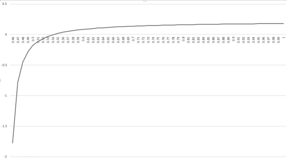
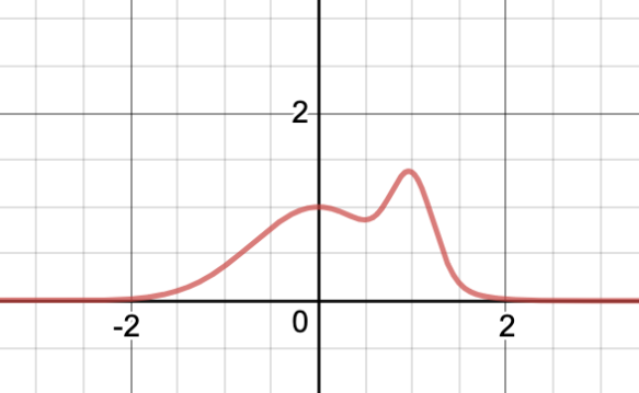
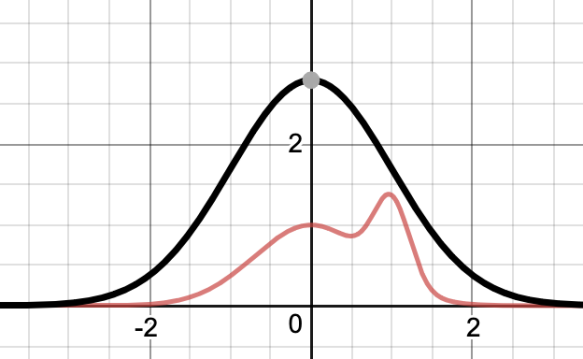
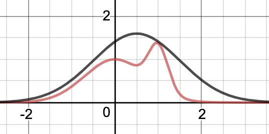
Aside: I’ve implemented the very useful gamma and beta distributions, but I won’t bother to show them in the blog. The code is tedious and explaining the mathematics would get us pretty off-topic. The short version is that the beta distribution is a distribution on numbers between 0 and 1 that can take on a variety of shapes. See the source code repository for the details of the implementation, and Wikipedia for an explanation of the distribution; various possible shapes for its two parameters are given below:

The code for the Beta and Gamma distributions and the rest of the code in this episode can be found here.

Let’s take Beta.Distribution(5, 5) as our prior distribution. That is, the “fairness” of the coins produced by our terrible mint is distributed like this:

var prior = Beta.Distribution(5, 5);
Console.WriteLine(prior.Histogram(0, 1));

                  ****                   
                 ******                 
                ********                
               **********               
               **********               
              ************              
              ************              
             **************             
             ***************            
            ****************            
            ****************            
           ******************           
          ********************          
          ********************          
         **********************         
        ***********************         
        ************************        
       **************************       
     ******************************     
----------------------------------------

Most of the coins are pretty fair, but there is still a significant fraction of coins that produce 90% heads or 90% tails.

We need a likelihood function, but that is easy enough. Let’s make an enumerated type for coins called Result with two values, Heads and Tails:

IWeightedDistribution<Result> likelihood(double d) => 
  Flip<Result>.Distribution(Heads, Tails, d);

We can use Metropolis to compute the posterior, but what should we use for the initial and proposal distributions? The prior seems like a perfectly reasonable guess as to the initial distribution, and we can use a normal distribution centered on the previous sample for the proposal.

IWeightedDistribution<double> posterior(Result r) =>
  Metropolis<double>.Distribution(
    d => prior.Weight(d) * likelihood(d).Weight(r), // weight
    prior, // initial
    d => Normal.Distribution(d, 1)); // proposal

But you know what, let’s once again make a generic helper function:

public static Func<B, IWeightedDistribution<double>> Posterior<B>(
  this IWeightedDistribution<double> prior,
  Func<double, IWeightedDistribution<B>> likelihood) =>
    b => 
      Metropolis<double>.Distribution(
        d => prior.Weight(d) * likelihood(d).Weight(b),
        prior,
        d => Normal.Distribution(d, 1));

And now we’re all set:

var posterior = prior.Posterior(likelihood);
Console.WriteLine(posterior(Heads).Histogram(0, 1));

                     ****               
                    ******              
                   *******              
                  *********             
                 ***********            
                ************            
                ************            
               *************            
               **************           
               ***************          
              ****************          
             ******************         
             ******************         
            *******************         
            ********************        
           **********************       
          ************************      
         *************************      
       *****************************    
----------------------------------------

It is subtle, but if you compare the prior to the posterior you can see that the posterior is slightly shifted to the right, which is the “more heads” end of the distribution.

Aside: In this specific case we could have computed the posterior exactly. It turns out that the posterior of a beta distribution in this scenario is another beta distribution, just with different shape parameters. But the point is that we don’t need to know any special facts about the prior in order to create a distribution that estimates the posterior.

Does this result make sense?

The prior is that a coin randomly pulled from this mint is biased, but equally likely to be biased towards heads or tails. But if we get a head, that is evidence, however slight, that the coin is not biased towards tails. We don’t know if this coin is close to fair, or very biased towards heads, or very biased towards tails, but we should expect based on this single observation that the first and second possibilities are more probable than the prior, and the third possibility is less probable than the prior. We see that reflected in the histogram.

Or, another way to think about this is: suppose we sampled from the prior many times, we flipped each coin exactly once, and we threw away the ones that came up tails, and then we did a histogram of the fairness of those that came up heads. Unsurprisingly, the coins more likely to turn up tails got thrown away more often than the coins that came up heads, so the posterior histogram is biased towards heads.

Exercise: Suppose we changed the scenario up so that we were computing the posterior probability of two flips. If we get two heads, obviously the posterior will be even more on the “heads” side. How do you think the posterior looks if we observe one head, one tail? Is it different than the prior, and if so, how? Try implementing it and see if your conjecture was correct.

What have we learned? That given a continuous prior, a discrete likelihood, and an observation, we can simulate sampling from the continuous posterior.

Why is this useful? The coin-flipping example is not particularly interesting, but of course coin-flipping is a stand-in for more interesting examples. Perhaps we have a prior on how strongly a typical member of a population believes in the dangers of smoking; if we observe one of them smoking, what can we deduce is the posterior strength of their beliefs? Or perhaps we have a prior on whether a web site user will take an action on the site, like buying a product or changing their password, or whatever; if we observe them taking that action, what posterior deductions can we make about their beliefs?

As we’ve seen a number of times in this series, it’s hard for humans to make correct deductions about posterior probabilities even when given good priors; if we can make tools available to software developers that help us make accurate deductions, that has a potentially powerful effect on everything from the design of developer tools to the design of public policy.

Next time on FAIC: Thus far in this series we’ve been very interested in the question “given a description of a distribution, how can I sample from it efficiently?” But there are other things we want to do with distributions; for example, suppose we have a random process that produces outcomes, and each outcome is associated with a gain or loss of some amount of money. What is the expected amount we will gain or lose in the long run? We’ll look at some of these “expected value” problems, and see how the gear we’ve developed so far can help compute the answers.

[It is] a spectacular vindication of the principle that each individual coin spun individually is as likely to come down heads as tails and therefore should cause no surprise that each individual time it does.

Thus Guildenstern (or is it Rosencrantz?) in Tom Stoppard’s re-imagining of Hamlet “Rosencrantz and Guildenstern Are Dead“. If you haven’t seen it already, go watch the movie, or at least the first scene.

It helps to know the plot of Hamlet: Before the play begins, prince Hamlet’s uncle Claudius has murdered Hamlet’s father, become king, and married Hamlet’s mother Gertrude. Hamlet is understandably perturbed by this sequence of events. Claudius and Gertrude have invited Hamlet’s college friends Rosencrantz and Guildenstern to cheer him up, but SPOILER ALERT in a series of misadventures they end up dead, soon to be followed by everyone else; the plot, such as it is, of R&G Are Dead is this story told from their confused, uninformed, and amnesiac perspective.

.

.

.

Welcome back. As you now know, if you did not before, Rosencrantz and Guildenstern are flipping (or, as they say, spinning) a series of coins. In the film sometimes they are flipping a different coin each time, which Rosencrantz (or is it Guildenstern?) wins, and sometimes they’re flipping the same coin several times in a row. Either way, the coin flipper (whatever his name is) hits an enormously unlikely sequence of heads.

Let’s make up a variation on this scenario to see what we can learn about posterior  distributions. (Code for this episode can be found here.)

Suppose we have two kinds of coins: fair, and double-headed. A fair coin has a 50-50 probability of coming up heads or tails; a double-headed coin always comes up heads.

enum Coin { Fair, DoubleHeaded }

Now let’s suppose we have a bag of coins. 999 are fair, and one is double-headed. Rosencrantz is going to pull a coin from the bag at random. Our prior is that the selection is random over the thousand coins in the bag, so:

var coins = new[] { Fair, DoubleHeaded };
var prior = coins.ToWeighted(999, 1);

Once he has his coin, Rosencrantz flips it, and of course, observes that it is heads.

The question I want to explore is: what is the posterior probability that Rosencrantz just flipped the double-headed coin?

That is, Rosencrantz draws a coin, flips it, it comes up heads, and now the question to you is: what would be fair odds for a bet on the question “is it the double-headed coin or a regular coin that was just flipped?” Prior to the observation the fair odds are 1 to 999, but after we observe the flip, those odds change because we have more information.

Reasoning backwards like this is a little tricky. (Of course we call it the posterior distribution because we are reasoning backwards, in case that was unclear.) Again, let’s break it down:

• Prior to flipping the coin, the probability of getting the double-headed coin is the aptly-named prior probability: 1 in 1000, which is odds of 1 to 999.
• If Rosencrantz flipped the coin and got tails, that would be solid evidence that he did not get the double-headed coin; the posterior probability of having the double headed coin is zero. That is, the posterior probability is smaller: we’ve gone from 0.1% to 0%, a small decrease.
• If Rosencrantz got heads, that is very weak evidence that he got a double-headed coin, but it is not zero evidence. There should be some small increase over the prior in the posterior.

Of course we don’t need to do the math by hand; we know from earlier in this series that we can exactly solve for posterior probabilities by using a combination of Where and SelectMany query operators:

var results = new[] { Heads, Tails };
IDiscreteDistribution<Result> likelihood(Coin c) =>
  results.ToWeighted(1, c == Fair ? 1 : 0);

var c1 = from c in prior
         from r in likelihood(c)
         where r == Heads
         select c;
Console.WriteLine(c1.ShowWeights());

        Fair:999
DoubleHeaded:2

If Rosencrantz flipped heads then the probability that he drew the double-headed coin is slightly increased over the prior. The prior probability of having the double-headed coin is 1 in 1000; the posterior probability is 2 in 1001. That’s almost twice as likely, but still pretty unlikely.

Again, let’s make sure that we understand what this means. It means that if we did millions of repetitions of this experiment where Rosencrantz picks a coin and flips it once, and if we discarded all the repetitions in which Rosencrantz flipped tails, then in the remaining repetitions on average the ratio of double-headed coins to fair coins chosen would be about 2 to 999.

What if we increase the number of flips of that same coin, and he got two heads?

var c2 = from c in prior
         from r1 in Likelihood(c)
         where r1 == Heads
         from r2 in Likelihood(c)
         where r2 == Heads
         select c;
Console.WriteLine(c2.ShowWeights());

        Fair:999
DoubleHeaded:4

The posterior probability of having the double-headed coin goes up again, this time to 4 in 1003.

What if we increased it to ten flips (again, of the same coin), and they’re all heads? By the time we get to ten heads, there are two possibilities: the exactly one-in-a-thousand chance that Rosencrantz got the double-headed coin, or the approximately one-in-a-thousand chance that he got a fair coin and flipped ten heads in a row; the ratio of those two probabilities is the posterior odds. At this point it becomes pretty much even money whether he has the double-headed coin or a fair coin. (As you might expect, the exact odds are 999 “fair” to 1024 “double-headed”, which is pretty darn close to 50-50.)

If we observe eleven or more heads, it becomes much more likely that Rosencrantz has drawn the one-in-a-thousand double-headed coin than that he is lucky enough to observe that sequence of heads from a fair coin, and of course by the time we get to 156 heads, it is absurdly more likely to be the double-headed coin than a fair coin.

This is a cute problem and all, but it seems a little out of place at this point in our series; we stopped talking about discrete distributions that we could solve exactly for posteriors a while back. I’m discussing it now because all this is in the way of introducing a variation on the above problem:

• We have a mint with really poor quality control; it produces coins that are out of balance, so that some of them favour heads and some of them favour tails.
• To model this, let’s say that the mint samples from some continuous distribution that produces values strictly between 0.0 and 1.0. Let’s say that we know this distribution.
• Each coin that is minted is modeled as a Bernoulli distribution of heads and tails, with the given probability of heads.
• Rosencrantz flips a random coin that was obtained from that mint; this is our prior.
• We observe that Rosencrantz gets heads.
• What is the posterior distribution on the fairness of that coin?

When I first started thinking about this problem I found it quite tricky to get it clear in my head, but this continuous version is not fundamentally different than the discrete version I gave above. In both cases we have a prior distribution of coin fairness that we sample from to get a coin. In both cases we then obtain an observation of “heads”. And in both cases, we can use that observation to deduce something about the likely provenance of the coin. Whether we’re in the continuous case or the discrete case, flipping heads is evidence that the coin is more likely to be on the “heads heavy” side of the prior distribution. But how much more likely?

In the all-discrete case we could compute that posterior exactly. The question before us now is: given the continuous prior, the discrete likelihood function and an observation of a discrete value, can we compute the weight function of the continuous posterior? That is, can we answer the question “what is the probable fairness level of this coin given that we’ve observed one head?” And of course, given all that information, can we also produce a distribution object that we can sample from?

Give it some thought.

Next time on FAIC: We will attempt to do so using the tools we’ve developed thus far.

Last time on FAIC we implemented a technique for sampling from a non-normalized target PDF:

• Find an everywhere-larger helper PDF that we can sample from.
• Sample from it.
• Accept or reject the sample via a coin flip with the ratio of weights in the target distribution and the helper distribution.

This technique totally works, but it has a few drawbacks:

• It’s not at all clear how to find a good helper PDF without humans intervening.
• Even with a pretty tight-fitting helper, you potentially still end up rejecting a lot of samples.

The first problem is the big one. It would be great if there was a technique that didn’t require quite so much intervention from experts.

Today I’ll describe just such a technique; it is called the “Metropolis algorithm” after one of its inventors, Nicholas Metropolis. [Code for this episode is here.]

Aside: The co-authors of the 1953 paper that first presented this algorithm are unfairly not credited in the name of the algorithm, but “the Metropolis algorithm” sounds snappy and cool, whereas “the Metropolis-Rosenbluth-Rosenbluth-Teller-and-Teller algorithm” is a bit of a mouthful.

In modern code we usually use a variation called the “Metropolis-Hastings algorithm“, but I’m not going to discuss it in this series.

Without further ado, here’s a sketch of the Metropolis algorithm:

• We have a non-normalized PDF f(t) that takes a T and returns a double. We want to produce arbitrarily many samples of T that conform to this distribution.
• The first time that Sample() is called we produce the initial sample.
• Now, obviously, if we could produce a random initial sample that matched the distribution described by f, we’d already have solved the problem! All that we require is a random initial sample that is somewhere in the support of f.
• We’ll call the distribution of the first sample the initial distribution.
• The initial sample becomes the current sample, which is returned.
• Every subsequent time that Sample() is called, we use the current sample to generate a candidate for the new sample; more specifically, we produce a proposal distribution of possible next samples.
• We sample the proposal distribution to get a proposed sample.
• We compute the weights f(current) and f(proposed)
• We divide the proposed weight by the current weight.
• If the quotient is greater than or equal to 1.0 then the proposed sample automatically becomes the new current sample.
• Otherwise, we flip a Bernoulli coin with that probability. Heads, we accept the proposed sample and it becomes the current sample. Tails, we keep the current sample.

Aside: Do you see why we don’t care if the PDFs are non-normalized in this algorithm? All we care about is the ratio of the weights when determining the Bernoulli distribution. Non-normalized PDFs have the same ratios as normalized PDFs!

Aside: There are a few technical restrictions on the proposal distribution that I’m not going to discuss; for details, see the Wikipedia page on ergodicity.

That might have been a bit abstract. Let’s say in type system terms what we need. First off, we have the target distribution we’re attempting to sample from:

Func<T, double> target;

Next, we have an initial distribution to get the first sample:

IDistribution<T> initial;

And finally, we have a function that produces proposal distributions:

Func<T, IDistribution<T>> proposals;

But… wait a minute. This looks really familiar.

• We’re producing a sequence of samples.
• We randomly choose an initial value.
• We randomly choose each subsequent value based on a probability distribution determined only by the previous value.

This is a Markov process!

Apparently we can use a Markov process to simulate sampling from an arbitrary PDF, assuming that the restrictions on the initial and proposal distributions are met.

Well this should be easy to implement, given that we’ve already implemented Markov processes, so let’s do it. This time, the fun will all be in the factory:

sealed class Metropolis<T> : IWeightedDistribution<T>
{
  private readonly IEnumerator<T> enumerator;
  private readonly Func<T, double> target;
  public static Metropolis<T> Distribution(
    Func<T, double> target, 
    IDistribution<T> initial, 
    Func<T, IDistribution<T>> proposal)
  {
    var markov = Markov<T>.Distribution(initial, transition);
    return new Metropolis<T>(
      target, markov.Sample().GetEnumerator());
    IDistribution<T> transition(T d)
    {
      T candidate = proposal(d).Sample();
      return Flip<T>.Distribution(
        candidate, d, target(candidate) / target(d));
    }
  }
  private Metropolis(
    Func<T, double> target,
    IEnumerator<T> enumerator)
  {
    this.enumerator = enumerator;
    this.target = target;
  }
  public T Sample()
  {
    this.enumerator.MoveNext();
    return this.enumerator.Current;
  }
  public double Weight(T t) => this.target(t);
}

Let’s try it out. We’ll need three things. For our target PDF, let’s take the mixed PDF we looked at last time:

double Mixture(double x) =>
  Exp(–x * x) + Exp((1.0 – x) * (x – 1.0) * 10.0);

What should our initial distribution be? All doubles are in the support of this distribution, so we can choose any, but we’d like it if the double was likely to be high-weight. Let’s suppose that we don’t know the exact shape of this distribution, but we do know that it has a lump near the origin, so we’ll just use a standard normal distribution as our initial value.

What should our proposal distribution be? It needs to be based on the current value, not biased to consistently get larger or smaller, and give us the possibility of any value in the support of our target distribution being produced. How about a normal distribution centered on the current value? That seems reasonable.

You know what, I’m going to make a helper method just for this case, since it seems likely to be pretty common:

public static Metropolis<double> NormalMetropolis(
    this Func<double, double> weight) =>
  Metropolis<double>.Distribution(
    weight,
    Normal.Standard,
    d => Normal.Distribution(d, 1.0));

Finally let’s run it and see if we get a reasonable histogram out:

NormalMetropolis(Mixture).Histogram(–2, 2)

                            ***         
                            ***         
                            ***         
                            ***         
                           *****        
                  ****     *****        
                 *******  ******        
                ******** *******        
               *****************        
              *******************       
             ********************       
            *********************       
            *********************       
           ***********************      
          ************************      
         *************************      
       ****************************     
      ******************************    
   **********************************   
----------------------------------------

Nice!

This seems to work really well, but unfortunately there are a few problems to deal with. Some of them are:

• We need an initial distribution that produces a value in the support. However, this is usually not too hard. And suppose by some accident we do end up getting a zero-weight element as the first sample; what’s going to happen? Probably the proposal distribution will pick a non-zero-weight element, and it will then automatically win, so hey, maybe the first sample is bad. No big deal.
• Let’s think a bit more about that issue though. Even if the first sample has positive weight, we might have a sequence of unusually low-weight samples at the beginning. If we start in a low-weight region there might be some time spent randomly walking around before we stumble into a high-weight region. Of course once we are in a high-weight region we are likely to stay there, which is good…
• … unless the distribution is “multimodal”. That is, there are multiple high-weight regions. Our example distribution in this episode is multimodal, but the two “lumps” are really close together and are “bridged” by a reasonable high-probability region; imagine a distribution where the “lumps” were far apart with a super-low-probability region between them. You can end up “stuck” in one of the lumps for a long time, and this can lead to situations where long sequences of samples have way more correlation between them than we would expect if we were sampling from the “real” distribution.
• The previous point is particularly emphasized by the fact that in a Metropolis simulation of sampling from a distribution, we frequently get repeated values in samples; that sort of correlation is typically not observed at all were we drawing from the “real” distribution rather than a Markovian simulation of it.

All of these problems can be dealt with by a variety of techniques; you’ve probably already thought of some of them:

• We could “burn” the first few dozen / hundred / whatever of the samples so that we get past any initial low-weight region.
• If samples are too correlated with each other, we could use a proposal distribution with a higher variance. (For example, we could use a normal distribution with a larger standard deviation.) That would increase the number of rejected samples, which increases repeats, but it would decrease the number of samples that were all close to each other but not rejections.
• Or, we could sample from a Bernoulli at a probability of our choosing on each sample, and if it’s heads, we skip enumerating the value but still keep it as our new state internally; that would decrease the amount of similarity between subsequent samples, while increasing the average computational cost of each sample.
• Or, we could generate samples in batches of a hundred or a thousand or whatever, randomly shuffle the batch, and then enumerate the shuffled batch, to decrease the amount of similarity between subsequent samples.

I’m not going to do any of these things, but I’m sure you can see how they would be done.

We’ve made really good progress here; we have an efficient general mechanism for sampling from a well-behaved PDF, so long as we have some idea of the initial distribution and a good guess at a proposal distribution. We also have some ideas for “tuning parameters” — that is, knobs that experts can turn to make tradeoffs between performance, correlation, and so on, and the knobs are simple enough that you could imagine writing a program to try different settings and figure out what works best.

Next time on FAIC: We’re going to seemingly take a step backwards and talk about a problem in discrete Bayesian reasoning: given a bag of coins, some unfair, and some observations of the results of flipping a coin pulled from the bag, what can we deduce about the coin we pulled?

Last time on FAIC we went through a loose, hand-wavy definition of what it means to have a “weighted” continuous distribution: our weights are now doubles, and given by a Probability Distribution Function; the probability of a sample coming from any particular range is the area under the curve of that range, divided by the total area under the function. (Which need not be 1.0.)

A central question of the rest of this series will be this problem: suppose we have a delegate that implements a non-normalized PDF; can we implement Sample() such that the samples conform to the distribution?

The short answer is: in general, no.

A delegate from double to double that is defined over the entire range of doubles has well over a billion billion possible inputs and outputs. Consider for example the function that has a high-probability lump in the neighbourhood of -12345.678 and another one at 271828.18 and is zero everywhere else; if you really know nothing about the function, how would you know to look there?

We need to know something about the PDF in order to implement Sample().

The long answer is: if we can make a few assumptions then sometimes we can do a pretty good job.

Aside: As I’ve mentioned before in this series: if we know the quantile function associated with the PDF then we can very easily sample from the distribution. We just sample from a standard continuous uniform distribution, call the quantile function with the sampled value, and the value returned is our sample. Let’s assume that we do not know the quantile function of our PDF.

Let’s look at an example. Suppose I have this weight function:

double Mixture(double x) =>
  Exp(–x * x) + Exp((1.0 – x) * (x – 1.0) * 10.0);

If we graph that out, it looks like this:

I called it “mixture” because it is the sum of two (non-normalized) normal distributions. This is a valid non-normalized PDF: it’s a pure function from all doubles to a non-negative double and it has finite area under the curve.

How can we implement a Sample() method such that the histogram looks like this?

Exercise: Recall that I used a special technique to implement sampling from a normal distribution. You can use a variation on that technique to efficiently sample from a mixture of normal distributions; can you see how to do so? See if you can implement it.

However, the point of this exercise is: what if we did not know that there was a trick to sampling from this distribution? Can we sample from it anyways?

The technique I’m going to describe today is, once more, rejection sampling. The idea is straightforward; to make this technique work we need to find a weighted “helper” distribution that has this property:

The weight function of the helper distribution is always greater than or equal to the weight function we are trying to sample from.

Now, remember, the weight function need not be “scaled” so that the area under the curve is 1.0. This means that we can multiply any weight function by a positive constant, and the distribution associated with the multiplied weight function is the same. That means that we can weaken our requirement:

There exists a constant factor such that the weight function of the helper distribution multiplied by the factor is always greater than or equal to the weight function we are trying to sample from.

This will probably be more clear with an example.

Let’s take the standard normal distribution as our helper. We already know how to sample from it, and we know it’s weight function. But it just so happens that there exists a constant — seven — such that multiplying the constant factor by the helper’s weight function dominates our desired distribution:

Again, we’re going to throw some darts and hope they land below the red curve.

• The black curve is the weight function of the helper — the standard normal distribution — multiplied by seven.
• We know how to sample from that distribution.
• Doing so gives us an x coordinate for our dart, distributed according to the height of the black curve; the chosen coordinate is more likely to be in a higher region of any particular width than a lower region of the same width.
• We’ll then pick a random y coordinate between the x axis and the black curve.
• Now we have a point that is definitely below the black line, and might be below the red line.
• If it is not below the red line, reject the sample and try again.
• If it is below the red line, the x coordinate is the sample.

Let’s implement it!

Before we do, once again I’m going to implement a Bernoulli “flip” operation, this time as the class:

sealed class Flip<T> : IWeightedDistribution<T>
{
  public static IWeightedDistribution<T> Distribution(
    T heads, T tails, double p)

You know how this goes; I will skip writing out all that boilerplate code. We take values for “heads” and “tails”, and the probability (from 0 to 1) of getting heads. See the github repository for the source code if you care.

I’m also going to implement this obvious helper:

static IWeightedDistribution<bool> BooleanBernoulli(double p) =>
  Flip<bool>.Distribution(true, false, p);

All right. How are we going to implement rejection sampling? I always begin by reasoning about what we want, and what we have. By assumption we have a target weight function, a helper distribution whose weight function “dominates” the given function when multiplied, and the multiplication factor. The code practically writes itself:

public class Rejection<T> : IWeightedDistribution<T>
{
  public static IWeightedDistribution<T> Distribution(
      Func<T, double> weight,
      IWeightedDistribution<T> helper,
      double factor = 1.0) =>
    new Rejection<T>(weight, dominating, factor);

I’ll skip the rest of the boilerplate. The weight function is just:

public double Weight(T t) => weight(t);

The interesting step is, as usual, in the sampling.

Rather than choosing a random number for the y coordinate directly, instead we’ll just decide whether or not to accept or reject the sample based on a Bernoulli flip where the likelihood of success is the fraction of the weight consumed by the target weight function; if it is not clear to you why that works, give it some thought.

public T Sample()
{
  while(true)
  {
    T t = this.helper.Sample();
    double hw = this.helper.Weight(t) * this.factor;
    double w = this.weight(t);
    if (BooleanBernoulli(w / hw).Sample())
      return t; 
  }
}

All right, let’s take it for a spin:

var r = Rejection<double>.Distribution(
  Mixture, Normal.Standard, 7.0);
Console.WriteLine(r.Histogram(–2.0, 2.0));

And sure enough, the histogram looks exactly as we would wish:

                             **         
                            ***         
                            ***         
                           *****        
                           *****        
                 ******   ******        
                ****************        
               *****************        
              *******************       
             ********************       
            *********************       
            *********************       
           ***********************      
          ************************      
         *************************      
        ***************************     
      *****************************     
    *********************************   
----------------------------------------

How efficient was rejection sampling in this case? Actually, pretty good. As you can see from the graph, the total area under the black curve is about three times the total area under the red curve, so on average we end up rejecting two samples for every one we accept. Not great, but certainly not terrible.

Could we improve that? Sure. You’ll notice that the standard normal distribution times seven is not a great fit. We could shift the mean 0.5 to the right, and if we do that then we can reduce the multiplier to 4:

That is a far better fit, and if we sampled from this distribution instead, we’d reject a relatively small fraction of all the samples.

Exercise: Try implementing it that way and see if you get the same histogram.

Once again we’ve managed to implement Sample() by rejection sampling; once again, what are the pros and cons of this technique?

• Pro: it’s conceptually very straightforward. We’re just throwing darts and rejecting the darts that do not fall in the desired area. The darts that do fall in the desired area have the desired property: that samples from a given area arrive in proportion to that area’s size.
• Con: It is by no means obvious how to find a tight-fitting helper distribution that we can sample such that the helper weight function is always bigger than the target weight function. What distribution should we use? How do we find the constant multiplication factor?

The rejection sampling method works best when we have the target weight function ahead of time so that we can graph it out and an expert can make a good decision about what the helper distribution should be. It works poorly when the weight function arrives at runtime, which, unfortunately, is often the case.

Next time on FAIC: We’ll look at a completely different technique for sampling from an arbitrary PDF that requires less “expert choice” of a helper distribution.