We now have enough gear to make a naïve “proto-QuickLife” implementation as a test to see (1) does it work at all? and (2) what is the performance compared to our other implementations at various levels of sophistication?

Code for this episode is here.

So far I’ve given you code for Quad2, Quad3, Quad4, the stepping algorithm for a Quad4 on even and odd cycles, and a lookup table to step even and odd Quad2s, so I won’t repeat that. What we need now is code to hold the whole thing together. I’ll omit a bunch of the code that does not relate directly to the task at hand, such as how we draw the screen, how we handle creating the initial pattern, and so on; see the source code link above if those algorithms interest you.

sealed class ProtoQuickLife : ILife, IReport
{
  // Number of 4-quads on a side.
  private const int size = 16;
  private int generation;
  private Dictionary<(short, short), Quad4> quad4s;

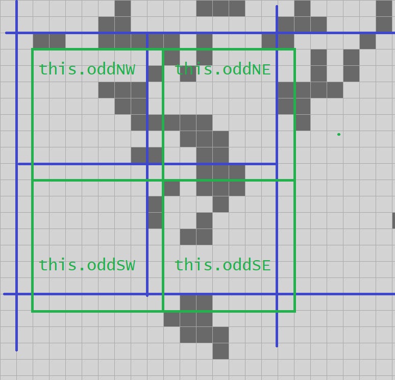
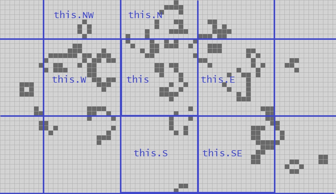
For our proto-QuickLife I’m just going to go with the same thing we saw in all of our previous fixed-size implementations: I’ll make an 8-quad. We have a 4-quad data structure in hand, and so we’ll need a 16 x 16 grid of 4-quads.

We need to know whether we are on an odd or even generation, so I’ve made a generation counter.

Since we have a fixed-size grid in this prototype version, I could just have an array of 256 Quad4s. However, in later versions of this algorithm we are going to use the sparse array technique I discussed in a previous episode, but it will be a sparse array of Quad4s, not cells! We’ll index our sparse array by a pair of shorts; that gives us a sparse 20-quad to play with, which is plenty of space; that’s a square with just over a million cells on a side. We might as well write the code for the sparse array now, and save having to write it again later.

public void Clear()
{
  generation = 0;
  quad4s = new Dictionary<(short, short), Quad4>();
  for (int y = 0; y < size; y += 1)
    for (int x = 0; x < size; x += 1)
      AllocateQuad4(x, y);
}

Some easy initialization code that allocates 256 Quad4s and puts them in a sparse array. A Quad4, recall, has six references to neighbouring Quad4s and everything else is a struct, so we will need to initialize those references; the structs will have their default values which, fortunately, is “all dead”.

private Quad4 AllocateQuad4(int x, int y)
{
  Quad4 c = new Quad4(x, y);
  c.S = GetQuad4(x, y - 1);
  if (c.S != null)
    c.S.N = c;
  ... and so on for N, E, W, SE, NW ...
  SetQuad4(x, y, c);
  return c;
}
private Quad4 GetQuad4(int x, int y)
{
  quad4s.TryGetValue(((short)x, (short)y), out var q);
  return q;
}
private void SetQuad4(int x, int y, Quad4 q) => 
  quad4s[((short)x, (short)y)] = q;

On all code paths to these private methods we will already know that the x, y coordinates are in bounds, so we have no problem casting them to shorts. I suppose there is some possibility that on the edges we will have “wrap around” behaviour for the additions and subtractions, but I’m not going to worry about it for the purposes of this blog.

And finally, the mainspring that drives the whole thing:

private bool IsOdd => (generation & 0x1) != 0;
public void Step()
{
  if (IsOdd)
    StepOdd();
  else
    StepEven();
  generation += 1;
}
private void StepEven()
{
  foreach (Quad4 q in quad4s.Values)
    q.StepEven();
}
private void StepOdd()
{
  foreach (Quad4 q in quad4s.Values)
    q.StepOdd();
}

Well that was all easy — as it should be, since the complicated work right now is in Quad4. (Don’t worry; this class will get much more complicated in coming episodes as we add optimizations.)

What do you think the time performance of this initial prototype is? Remember, this is a fully naïve implementation in the sense that we are not doing any kind of change tracking, we are not identifying “all dead” Quad4s and skipping them, and so on. We have a 256×256 grid and we are computing the next generation by looking at every one of those cells; the optimization we have with our lookup table is that we compute the results “four at a time” via lookup to get a 1-quad rather than by counting neighbours.

To get an apples-to-apples comparison I ran the proto-QuickLife algorithm using the same test as we’ve done so far in this series: 5000 ticks of “acorn” on an 8-quad. Make a guess, and then scroll down for the results.

.

.

.

.

.

.

Algorithm           time(ms)  ticks  size(quad)    megacells/s
Naïve (Optimized):   4000       5K      8               82
Abrash (Original)     550       5K      8              596
Stafford              180       5K      8             1820
Proto-QuickLife       770       5K      8              426

A considerable improvement over the original naïve algorithm, but unsurprisingly, not as fast as our more optimized solutions.

What about memory? In this prototype implementation we have 65536 cells, and we are storing two generations. How many bits are we using? (We will ignore fixed costs such as the lookup tables.) If we suppose that references are 8 bytes then:

• A Quad2 is exactly 2 bytes
• A Quad3 is exactly 8 bytes
• A Quad4 has eight Quad3s, so 64 bytes for the data, plus 4 bytes for the coordinates, plus 48 bytes for the references, plus another 4 bytes for the object header maintained by the runtime. That’s 120 bytes per Quad4. Oh, and our sparse array has an overhead of at minimum 12 bytes per entry, since an entry is two shorts and a reference, so call it 132 bytes all up.
• We’ve got 256 Quad4s in this implementation, so that’s 33792 bytes to represent 65536 cells, or just slightly over four bits per cell.

That’s not bad; recall that Stafford’s algorithm was 5 bits per cell.

We are off to a good start here.

Coming up on FAIC:

We’ve created a solid foundation for adding more optimizations and features. In the next few episodes we will explore these questions:

• As we have seen several times already in this series, if we identify what cells are changing then we can spend time on only those cells. Can we use the fact that we are storing two generations worth of cells in each Quad4 to make an even better change-tracking optimization?
• Even if we eliminate the time cost, an all-dead Quad4 with all-dead neighbours seems like it is taking up space unnecessarily. Can we efficiently prune all-dead Quad4s from the sparse array and save on that space?
• If we have robust change tracking then we can discover changing cells that border a “missing” Quad4. Can we grow the set of Quad4s dynamically as a pattern expands into new space, and thereby achieve Life on an 20-quad?

We’re continuing with our deep dive into Alan Hensel’s QuickLife algorithm, rewritten in C# with an emphasis on clarity. When last we left off we had the following established:

• A Quad2 is an immutable wrapper around a ushort
• A Quad3 is an immutable struct containing four Quad2s
• A Quad4 is a mutable class containing eight Quad3’s; four for the even generations and four for the odd, plus references to the Quad4s to the north, south, east, west, northwest and southeast.
• The odd generation is “one cell to the southeast” of the even generation.
• We have an algorithm that efficiently steps the even generation (blue) to the odd generation (green):

How then are we going to step the odd generation back to the even generation? If stepping the even generation produces an odd generation that is “one to the southeast” then stepping the odd generation in the same way will also go “one to the southeast”.

Long-time reader svick pointed out in a comment to the previous episode that maybe that’s not so bad! If our coordinate system has to shift “one to the southeast” every step then we could do things like adding new Quad4s to the north and west edges every sixteen ticks, and remove old ones from the south and east edges, and on average we would stay “in the same place”.

I would love to experiment with that idea, but I want to stay on target more. The QuickLife algorithm uses the fact that we alternate between “one to the southeast” and “one to the northwest” to attain optimizations that we will see in later episodes.

Plainly then what we must do is write the equivalent algorithm that goes “one to the northwest.” Let’s attack the problem just on the Quad3 I’ve labeled “this.oddSE” to start with.

Two episodes ago we made a method that takes nine Quad2s and returns a Quad3. I’m going to rename that method to Step9Quad2ToQuad3Even because it only works on evens. I won’t go through the same level of exegesis that I did the first time around as we write…

static Quad3 Step9Quad2ToQuad3Odd(
  Quad2 nw, Quad2 n, Quad2 ne,
  Quad2 w, Quad2 c, Quad2 e,
  Quad2 sw, Quad2 s, Quad2 se)
{

What information do we need to get a Quad3 that is one tick ahead and one cell to the northwest?

We can get a quarter of the information we need by looking up the next generation centers of the center, east, south and southeast 2-quads; the cells for the next even generation that we can compute from the green 2-quads is show by blue 1-quads:

The blue 1-quads will be the southeast corners of the four next-generation 2-quads.

We can get another quarter by getting these “mirrored” Quad2s:

  Quad2 c_e = c.HorizontalMiddleMirrored(e);
  Quad2 s_e = s.HorizontalMiddleMirrored(se);
  Quad2 c_w = w.HorizontalMiddleMirrored(c);
  Quad2 s_w = sw.HorizontalMiddleMirrored(s);

and then use a lookup table to get this state:

That gives us the southwest corners of the four next-generation Quad2s.

We can get these “flipped” Quad2s:

  Quad2 c_s = c.VerticalMiddleFlipped(s);
  Quad2 e_s = e.VerticalMiddleFlipped(se);
  Quad2 c_n = n.VerticalMiddleFlipped(c);
  Quad2 e_n = ne.VerticalMiddleFlipped(e);

to get this state:

for the northeast corners.

And finally we can get these “mirrored and flipped” Quad2s:

  Quad2 c_ne = c_n.HorizontalMiddleMirrored(e_n);
  Quad2 c_sw = c_w.VerticalMiddleFlipped(s_w);
  Quad2 c_se = c_s.HorizontalMiddleMirrored(e_s);
  Quad2 c_nw = c_w.NorthEdge | c_n.SW | nw.SE;

to get this state:

for the northwest corners of each new Quad2.

Putting it together, we can get this information:

As desired, the next step is a Quad3 “one to the northwest” from the Quad3 formed by the center, east, south and southeast Quad2s.

We haven’t yet written the code to actually do the lookups and generate the four Quad2s, but we can just use the same lookup tables as last time…

Wait a minute. No, we cannot!

Remember how we arranged our lookup table? We noticed the following facts for the even-to-odd cycle, which we then made use of in designing the lookup table:

• The next-tick 1-quads that go in the NW corner of a Quad2 are generated by stepping a “normal” Quad2.
• The 1-quads that go in the SW corner are generated by stepping a “flipped” Quad2.
• The 1-quads that go in the NE corner are generated by stepping a “mirrored” Quad2.
• The 1-quads that go in the SE corner are generated by stepping a flipped and mirrored Quad2.

Are any of those conditions still met?  Sadly no. If you look carefully you’ll see that we are now in the opposite situation. On the odd-to-even cycle:

• The next-tick 1-quads that go in the SE corner of a Quad2 are generated by stepping a “normal” Quad2.
• The 1-quads that go in the NE corner are generated by stepping a “flipped” Quad2.
• The 1-quads that go in the SW corner are generated by stepping a “mirrored” Quad2.
• The 1-quads that go in the NW corner are generated by stepping a flipped and mirrored Quad2.

What are we going to do about this? We could solve the problem by doing a bunch of bit shifting, but remember that the whole point of our technique of storing the “next generation” 1-quads in a lookup table at the bit positions where they are going to be needed is to avoid that bit shifting by moving it back in time to the generation of the table.

I’m sure you see the obvious solution: build a second lookup table that has the properties that we want! It’s only an additional 128K of memory.

Something we will see as we continue porting the QuickLife algorithm to C# is that the whole thing is based on the even and odd cycles being almost the same but different enough that you end up writing all the code twice. There will be a lot of duplicated code in my implementation, and my implementation will have quite a bit less duplication than the original.

So we’ll make two lookup tables, one for even and one for odds; I’ll omit the generation of the odd lookup table because it is just like the even lookup table, just with the results put in different bit positions. Our function for today then ends just as you’d expect:

  Quad2 newNW = OddLookup(c).SE | OddLookup(c_n).NE | OddLookup(c_w).SW | OddLookup(c_nw).NW;
  Quad2 newNE = OddLookup(e).SE | OddLookup(e_n).NE | OddLookup(c_e).SW | OddLookup(c_ne).NW;
  Quad2 newSW = OddLookup(s).SE | OddLookup(c_s).NE | OddLookup(s_w).SW | OddLookup(c_sw).NW;
  Quad2 newSE = OddLookup(se).SE | OddLookup(e_s).NE | OddLookup(s_e).SW | OddLookup(c_se).NW;
  return new Quad3(newNW, newNE, newSW, newSE);
}

That takes care of the problem of “get the next Quad3 given nine Quad2s”. Last time we described how to use that helper function to step an even-to-odd Quad4, and again it should come as no surprise that odd-to-even is just the same except slightly different:

public void StepOdd()
{
  StepOddSE();
  StepOddNW();
  StepOddSW();
  StepOddNE();
}
private void StepOddSE()
{
  evenSE = Step9Quad2ToQuad3Odd(
    oddNW.SE, oddNE.SW, oddNE.SE,
    oddSW.NE, oddSE.NW, oddSE.NE,
    oddSW.SE, oddSE.SW, oddSE.SE);
}
private void StepOddNW()
{
  evenNW = Step9Quad2ToQuad3Odd(
    NW == null ? AllDead : NW.oddSE.SE,
    N == null ? AllDead : N.oddSW.SW,
    N == null ? AllDead : N.oddSW.SE,
    W == null ? AllDead : W.oddNE.NE,
    oddNW.NW,
    oddNW.NE,
    W == null ? AllDead : W.oddNE.SE,
    oddNW.SW,
    oddNW.SE);
}
...

And so on; I won’t write them all out here.

Once again I have four methods that have just one method call in them each because in future episodes we will be adding more stuff here.

Next time on FAIC: We now have enough gear that we can write a simple working “proto-QuickLife” algorithm that steps a fixed set of Quad4s. We’ll do that, take a look at its performance, and then think about ways to build a much faster, much more memory-efficient, and much more dynamic implementation on top of the foundation we’ve built so far.

For today’s extra content:

We’ve already seen the four smallest spaceships (glider, and the three variants of light/middle/heavy spaceship). “Loafer” is the fifth smallest spaceship, and moves at a relatively leisurely c/7. It’s called loafer because of this slow pace and because it appears to be pushing a loaf still Life ahead of it. (Once again for reasons unknown WordPress is not serving up the animation, so see the wiki for the animation or click here.)

Last time on FAIC we saw how we could start with nine 2-quads — a 12×12 grid of cells — and with only a handful of ands, ors and table lookups we could get an 8×8 grid of cells of the next state out. How is that useful?

In order to explain, we need two more data structures, and it should come as no surprise that they are Quad3 and Quad4. Quad3, as I mentioned last time, is trivial; it is just a struct wrapping four Quad2s. The implementation is simpler than Quad2:

struct Quad3
{
  public Quad3(Quad2 nw, Quad2 ne, Quad2 sw, Quad2 se)
  {
    NW = nw;
    NE = ne;
    SW = sw;
    SE = se;
  }
  public Quad2 NW { get; }
  public Quad2 NE { get; }
  public Quad2 SW { get; }
  public Quad2 SE { get; }
  public bool Get(int x, int y) { ... }
  public Quad3 Set(int x, int y) { ... }
  public Quad3 Clear(int x, int y) { ... }
  public override string ToString() { ... }
}

We have yet another immutable struct. It’s small — only 64 bits. The Get, Set, Clear and ToString implementations are the obvious and straightforward extensions of the similar methods I already showed for Quad2, so I won’t bother showing them here. In a few episodes we will need to add some helper methods to Quad3, but for now, this will do us just fine.

The interesting data structure is Quad4, which by rights should represent a 16×16 grid of cells. The Quad4 has some surprises:

• A Quad4 is a mutable class, not an immutable struct.
• A Quad4 is not four Quad3s. It is eight! A Quad4 represents two ticks worth of a 16×16 portion of the grid. We have four Quad3s for the even-numbered generations, and four for the odds.
• Each Quad4 is numbered with a unique (x, y) pair of signed short integers. That gives us a square of Quad4s 65536 on a side; since each Quad4 is 16 cells wide and tall, we have a total grid size of just over one million cells on a side; that’s a 20-quad. That’s pretty big. Of course, we will typically allocate nowhere even close to that many Quad4s.
• Each Quad4 has a reference to six neighbouring Quad4s; specifically, it knows what Quad4s are to its north, south, west, east, northwest and southeast. A null reference is to be treated as though those cells are all dead. (Why not northeast and southwest? We shall see.)

There are more surprises to come later. Let’s write some code. It’s pretty straightforward:

sealed class Quad4
{
  public Quad4(int x, int y)
  {
    X = (short)x;
    Y = (short)y;
  }

  // A unique pair of shorts for each 4-quad in a 20-quad.
  public short X { get; }
  public short Y { get; }

  // References to neighbouring Quad4s:
  public Quad4 N { get; set; }
  public Quad4 S { get; set; }
  public Quad4 E { get; set; }
  public Quad4 W { get; set; }
  public Quad4 NW { get; set; }
  public Quad4 SW { get; set; }

  // Cells
  private Quad3 evenNW;
  private Quad3 evenSW;
  private Quad3 evenNE;
  private Quad3 evenSE;
  private Quad3 oddNW;
  private Quad3 oddSW;
  private Quad3 oddNE;
  private Quad3 oddSE;

  public bool GetEven(int x, int y) { ... }
  public void SetEven(int x, int y) { ... }
  public void ClearEven(int x, int y) { ... }

  public bool GetOdd(int x, int y) { ... }
  public void SetOdd(int x, int y) { ... }
  public void ClearOdd(int x, int y) { ... }

  public string override ToString() { ... }
}

Once again those last seven methods are (for now!) just trivial rewrites of the equivalent methods on a Quad2, so I’ll omit them here.

Obviously some controlling code representing the entire grid needs to create some number of Quad4s, assign numbers to them, set up the references, and so on. We’ll write that code in a later episode; right now I want to continue concentrating on the key problem of stepping to the next tick.

Suppose we are currently on an even generation and we want to step all the Quad4s in the system to the next generation, which will of course be odd. We add this method to Quad4 and have the controlling code call it for every Quad4:

public void StepEven()
{
  StepEvenNW();
  StepEvenSW();
  StepEvenNE();
  StepEvenSE();
}

Pretty straightforward; we step every even Quad3 forward one tick, and presumably that fills in the odd Quad3s. How are we going to do that though?

Time for more diagrams.

Again I’ve just randomly chosen a fragment of “acorn”, this time from generation 416. Let’s suppose the 4-quad I’ve marked as “this” is the one we are attempting to step forward one generation. (Click on any image for a higher-res version if one is available.)

Let’s zoom in a bit on “this” and give expressions that refer to some interesting Quad2s:

Well would you look at what we have here: nine Quad2s. If we step those forward one step with our handy super-efficient method from last episode, we get the next state of the green Quad3:

The code could not be easier:

private void StepEvenNW()
{
  oddNW = Step9Quad2ToQuad3(
    evenNW.NW, evenNW.NE, evenNE.NW,
    evenNW.SW, evenNW.SE, evenNE.SW,
    evenSW.NW, evenSW.NE, evenSE.NW);
}

I’m going to keep this in its own method though, as I’ll be adding more gear to it in an upcoming episode.

That’s the easy one, and I don’t think I need to labour the point with more diagrams. In order to step forward the other Quad3s we need to be careful about the fact that this.E, this.SE and this.S could be null, but if they are, we just substitute in an all-dead Quad2, which we helpfully made a static field for last time:

private void StepEvenSW()
{
  oddSW = Step9Quad2ToQuad3(
    evenSW.NW, evenSW.NE, evenSE.NW,
    evenSW.SW, evenSW.SE, evenSE.SW,
    S == null ? AllDead : S.evenNW.NW,
    S == null ? AllDead : S.evenNW.NE,
    S == null ? AllDead : S.evenNE.NW);
}
private void StepEvenNE()
{
  oddNE = Step9Quad2ToQuad3(
    evenNE.NW, evenNE.NE, E == null ? AllDead : E.evenNW.NW,
    evenNE.SW, evenNE.SE, E == null ? AllDead : E.evenNW.SW,
    evenSE.NW, evenSE.NE, E == null ? AllDead : E.evenSW.NW);
}
private void StepEvenSE()
{
  oddSE = Step9Quad2ToQuad3(
    evenSE.NW, evenSE.NE, E == null ? AllDead : E.evenSW.NW,
    evenSE.SW, evenSE.SE, E == null ? AllDead : E.evenSW.SW,
    S == null ? AllDead : S.evenNE.NW,
    S == null ? AllDead : S.evenNE.NE,
    SE == null ? AllDead : SE.evenNW.NW);
}

And when StepEven returns, we have the next state for the odd generation:

Wait a minute. We have committed the classic programmer blunder of being consistently off by one! We haven’t computed the next generation of the even 4-quad; we’ve computed the next generation of the 4-quad that is the even 4-quad shifted one cell to the southeast.

Well golly.

What are we going to do about this?

Give that some thought and then scroll down.

.

.

.

.

.

.

.

In my youth I was in a group of friends that watched terrible 80s horror movies every week, and we noticed patterns. In particular, in Killer Mutant Critter movies and zombie movies there is often a sheriff, and there are often concerned townsfolk, and the dialog seems to go

“Sheriff! Giant mutant toads are attacking the village! What are you going to do about it?!”

“Nuthin’.”

That’s what we’re going to do about it. Nuthin’.

This is our final surprise for this episode. A Quad4 represents a 16×16 section of the grid, for two generations, where the odd numbered generation is offset by one cell to the southeast from the even generation. Though this will make life very slightly difficult for the display code, this “staggered generations” property turns out to be surprisingly useful; we will see why in an upcoming episode.

Next time on FAIC: The next problem we need to solve is: how are we going to do the odd generation steps? We can’t just do the same thing because then we’ll be two cells off. Somehow we need to have the odd step get back to the northwest.

Let’s crisp up the problem from last episode. The problem for today’s episode is to write a method that takes these nine 2-quads:

Computes these sixteen 1-quads:

And returns these four 2-quads:

Those four 2-quads form a 3-quad; I haven’t written a 3-quad data structure yet, but I’m sure you can imagine how it goes. We’ll write it out later; it’s just a struct containing four 2-quads. I like to start by writing the signature of the method:

static Quad3 Step9Quad2ToQuad3(
  Quad2 nw, Quad2 n, Quad2 ne,
  Quad2 w, Quad2 c, Quad2 e,
  Quad2 sw, Quad2 s, Quad2 se)
{

The first step is to get those twelve additional 2-quads. The first four we need are these:

Start at the beginning: how are we going to get the western 2-quad on the northern edge? Plainly it is made up of parts of the 2-quads I’ve labeled NW and N. A couple episodes ago I added an “or” operator to 2-quads and masks that get the eastern and western edges, so how about this?

Quad2 n_w = nw.EastEdge | n.WestEdge;

Do you see why that’s not quite right?  That is this 2-quad:

We’ve pasted the east edge of nw and the west edge of n together, but we also need to swap eastness with westness. The result we’ve got is mirror-imaged-at-the-level-of-1-quads the 2-quad that we want. Make sure that this step is clear in your head because correctly understanding how this is “mirrored” is important in this algorithm.

We’re going to be doing these operations a lot in this episode, so in keeping with my general attitude of “there’s nothing too small to go in a method”, I’m going to make two helper methods on Quad2 right now; one creates a problem and one fixes it:

public Quad2 HorizontalMiddleMirrored(Quad2 right) =>
  EastEdge | right.WestEdge;
public Quad2 Mirror =>
  new Quad2((ushort)((cells << 8) | (cells >> 8)));

Now we can write correct code for extracting the n_w 2-quad:

Quad2 n_w = nw.HorizontalMiddleMirrored(n).Mirror;

Why not combine these into one helper function HorizontalMiddle? Normally I would, but… we will come back to this point in a bit.

So far we’ve done two ands, two ors and two shifts. We can do three times that work to similarly get:

Quad2 n_e = n.HorizontalMiddleMirrored(ne).Mirror;
Quad2 c_w = w.HorizontalMiddleMirrored(c).Mirror;
Quad2 c_e = c.HorizontalMiddleMirrored(e).Mirror;

We now have eight of the sixteen 2-quads that we need. I’m sure you see how we can get these four:

We need to do the same thing again but this time for the vertical direction. And this time the 2-quads are going to come out flipped north-for-south instead of mirrored east-for-west. Two more helper methods!

public Quad2 VerticalMiddleFlipped(Quad2 bottom) =>
  SouthEdge | bottom.NorthEdge;
public Quad2 Flip => 
  new Quad2((ushort)(((cells & SouthEdgeMask) << 4) | 
    ((cells & NorthEdgeMask) >> 4)));

and now we can compute those four:

Quad2 w_n = nw.VerticalMiddleFlipped(w).Flip;
Quad2 w_s = w.VerticalMiddleFlipped(sw).Flip;
Quad2 c_n = n.VerticalMiddleFlipped(center).Flip;
Quad2 c_s = center.VerticalMiddleFlipped(s).Flip;

We’re 75% of the way to getting our sixteen needed 2-quads. How are we going to get these?

Three of them are pretty easy; they can be constructed from what we already have in hand.

Quad2 c_nw = w_n.HorizontalMiddleMirrored(c_n).Mirror;
Quad2 c_sw = w_s_flip.HorizontalMiddleMirrored(c_s).Mirror;
Quad2 c_ne = n_e.VerticalMiddleFlipped(c_e).Flip;

That last one is a little tricky but we can get it:

Quad2 s_e = s.HorizontalMiddleMirrored(se).Mirror;
Quad2 c_se = c_e.VerticalMiddleFlipped(s_e).Flip;

So far we’ve done 26 each of and, or, shift, to get the 16 2-quads we need.

We supposed that we had a fast lookup table that took a 2-quad and returned a 1-quad; let’s actually build that. The 2-quad key is a ushort and the returned 1-quad is an integer where the low four bits are the bits of the 1-quad:

static int[] lookup = new int[65536];
... initialized as ...
for (int i = 0; i <= 0xffff; i += 1)
  lookup[i] = StepQuad2(new Quad2((ushort)i));

We can therefore solve our problem with this mess:

Quad2 newNW = new Quad2((ushort)(
  (lookup[(ushort)nw] << 12) | // NW is bits 12-15
  (lookup[(ushort)w_n] << 8) | // SW is 8-11
  (lookup[(ushort)n_w] << 4) | // NE is 4-7
  (lookup[(ushort)c_nw])));    // SE is 0-3
Quad2 newNE = new Quad2((ushort)(
  (lookup[(ushort)n] << 12) |
  (lookup[(ushort)c_n] << 8) |
  (lookup[(ushort)n_e] << 4) |
  (lookup[(ushort)c_ne])));
Quad2 newSW = new Quad2((ushort)(
  (lookup[(ushort)w] << 12) |
  (lookup[(ushort)w_s] << 8) |
  (lookup[(ushort)c_w] << 4) |
  (lookup[(ushort)c_sw])));
Quad2 newSE = new Quad2((ushort)(
  (lookup[(ushort)c] << 12) |
  (lookup[(ushort)c_s] << 8) |
  (lookup[(ushort)c_e] << 4) |
  (lookup[(ushort)c_se])));
return new Quad3(newNW, newNE, newSW, newSE);

What I like about this: it would work.

What I dislike about this: we’re back in the mechanism domain. We are treating 1-quads as ints and constantly going back and forth between ushorts and Quad2s. The implementation detail of how a Quad2 is laid out in memory is once again front and center in this algorithm. Also, it feels like we are doing more work than we need to throughout this algorithm.

And we are wasting a bunch of space in the lookup table. We have 65536 32-bit integers but we are only using 4 of those bits. That seems like a small problem; memory is cheap after all but… wait a minute… what if we could fix several of these problems at once?

The first step in fixing this mess is: we’re going to make the lookup table an array of Quad2s, where each Quad2 contains four copies of the 1-quad:

static Quad2[] lookup = new Quad2[65536];
... initialized as ...
for (int i = 0; i <= 0xffff; i += 1)
{
  int n = StepQuad2(new Quad2((ushort)i));
  lookup[i] = new Quad2((ushort)(
    (n << 12) | (n << 8) | (n << 4) | n));
}
...
static Quad2 Lookup(Quad2 q) => lookup[(ushort)q];

I mean, why not? We have plenty of bits to spare, so use them.

Now the call site looks like this:

Quad2 newNW =  Lookup(nw).NW | Lookup(w_n).SW | Lookup(n_w).NE | Lookup(c_nw).SE;
Quad2 newNE =  Lookup(n).NW  | Lookup(c_n).SW | Lookup(n_e).NE | Lookup(c_ne).SE;
Quad2 newSW =  Lookup(w).NW  | Lookup(w_s).SW | Lookup(c_w).NE | Lookup(c_sw).SE;
Quad2 newSE =  Lookup(c).NW  | Lookup(c_s).SW | Lookup(c_e).NE | Lookup[c_se].SE;
return new Quad3(newNW, newNE, newSW, newSW);

Look at that improvement in the readability of the code! We plainly see that we are constructing new Quad2s out of the parts of old ones. We’re keeping all the typing consistent. This is great.

Could it be even better?

Take a look at those sixteen computations of a quad1 on the next tick. You notice something?

• All the ones that are going in the NW of a new 2-quad are lookups on an argument that was passed in to this method: nw, n, w and c.
• All the ones that are going to the SW were computed by “flipping” something: w_n, c_n, w_s and c_s.
• All the ones that are going to the NE were computed by “mirroring” something: n_w, n_e, c_w and c_e
• All the ones going to the SE were both flipped and mirrored: c_nw, c_ne, c_sw, c_se.

What does this mean?

It means we can move the flipping and mirroring operations back in time into the lookup table as well. Read this next bit carefully because it is tricky. We’re going to initialize the lookup table like this:

for (int i = 0; i <= 0xffff; i += 1)
{
  Quad2 normal = new Quad2((ushort)i);
  Quad2 mirror = normal.Mirror;
  Quad2 flip = normal.Flip;
  Quad2 both = mirror.Flip;
  int result = StepQuad2(normal);
  lookup[(ushort)both] |= new Quad2((ushort)result);           // SE
  lookup[(ushort)mirror] |= new Quad2((ushort)(result << 4));  // NE
  lookup[(ushort)flip] |= new Quad2((ushort)(result << 8));    // SW
  lookup[(ushort)normal] |= new Quad2((ushort)(result << 12)); // NW
}

And now we can remove all the flips and mirrors when computing the new Quad2s! Put it all together:

static Quad3 Step9Quad2ToQuad3(
  Quad2 nw, Quad2 n, Quad2 ne,
  Quad2 w, Quad2 c, Quad2 e,
  Quad2 sw, Quad2 s, Quad2 se)
{
  // These are mirrored
  Quad2 n_w = nw.HorizontalMiddleMirrored(n);
  Quad2 n_e = n.HorizontalMiddleMirrored(ne);
  Quad2 c_w = w.HorizontalMiddleMirrored(c);
  Quad2 c_e = c.HorizontalMiddleMirrored(e);
  // These are flipped
  Quad2 w_n = nw.VerticalMiddleFlipped(w);
  Quad2 c_n = n.VerticalMiddleFlipped(c);
  Quad2 w_s = w.VerticalMiddleFlipped(sw);
  Quad2 c_s = c.VerticalMiddleFlipped(s);
  // These are mirrored and flipped
  Quad2 c_nw = w_n.HorizontalMiddleMirrored(c_n);
  Quad2 c_ne = n_e.VerticalMiddleFlipped(c_e);
  Quad2 c_sw = w_s.HorizontalMiddleMirrored(c_s);
  Quad2 c_se = c_e.SouthEdge | c_s.NE | se.NW;
  Quad2 newNW =  Lookup(nw).NW | Lookup(w_n).SW | Lookup(n_w).NE | Lookup(c_nw).SE;
  Quad2 newNE =  Lookup(n).NW  | Lookup(c_n).SW | Lookup(n_e).NE | Lookup(c_ne).SE;
  Quad2 newSW =  Lookup(w).NW  | Lookup(w_s).SW | Lookup(c_w).NE | Lookup(c_sw).SE;
  Quad2 newSE =  Lookup(c).NW  | Lookup(c_s).SW | Lookup(c_e).NE | Lookup[c_se].SE;
  return new Quad3(newNW, newNE, newSW, newSW);
}

Computing c_se actually gets easier, which is a nice bonus.

What’s our final tally? To move ahead an 8×8 portion of a 12×12 grid we do 41 ands, 25 ors and 16 array lookups. And zero shifts. All the other bit operations have been moved backwards in time to run during the computation of the lookup table.

Could we do even less work?

Yes; we could eliminate 16 of those ands if we had four lookup tables each with four bits in the right place and zeros everywhere else; we then would not have to do any masking. It would just be:

  Quad2 newNW =  LookupNW(nw) | LookupSW(w_n) | LookupNE(n_w) | LookupSE(c_nw);
  ...

But that’s not how the original implementation did it, and so that’s not what I’m doing here. It would be an interesting experiment to find out of that makes a difference; maybe we will come back to that point later in the series, but probably not.

Oh, and incidentally, you remember that fragment of bit-twiddling code that I posted from the original implementation?

int ix01 = (ix00 & 0xf0f0) | (cN.q[14] & 0x0f0f);
int ix11 = (ix10 & 0xf0f0) | (cN.q[15] & 0x0f0f);
int ix03 = (ix02 & 0xf0f0) | (ix01 & 0x0f00) | (cN.q[7] & 0x000f);

I bet you can figure out what it does now!

Well that was quite the journey to get a fast method that can step an 8×8 fragment of a 12×12 grid forwards one tick by memoizing the “4×4 step to 2×2” problem. Why is this method useful?

Next time on FAIC: Yeah, why?

When last we left off we had representations for 0-quads — a single bit — 1-quads — four bits in a row — and 2-quads — a wrapper data structure around an unsigned short that could extract single cells or mask out any of the component 1-quads “in place”. The question in the cliffhanger was: how can we move a 2-quad — a 4×4 grid of cells — forwards one generation?  Should we just pretend that there is a rectangle of empty cells around it?

No. Instead, we redefine what it means to step one tick forward. Stepping a 2-quad forward one tick results in a 1-quad; the center one-quad stepped one tick forwards.

Let me make sure that’s clear. What I’m saying is that if we have this 2-quad, just to pick one at random:

And we step it forwards one tick, we assume that this 2-quad is embedded in a larger grid and we do not know the true neighbour counts of the twelve cells on the edge. But we do have enough information to step the center four cells forwards, and that gives us a 1-quad:

The implementation is straightforward; we’ve seen it a bunch of times. Since I don’t have a custom-built data structure for a 0-quad or a 1-quad and they are just one bit or four bits, let’s just put them in an integer and we’ll figure out what to do with them later. (Recall that I said that bits 3, 2, 1, and 0 were the northwest, northeast, southwest and southeast cells of a 1-quad.)

private static int Rule(int cell, int count)
{
  if (count == 2)
    return cell;
  if (count == 3)
    return 1;
  return 0;
}
private static int StepQuad2(Quad2 q)
{
  int b00 = q.Get(0, 0) ? 1 : 0;
  int b01 = q.Get(0, 1) ? 1 : 0;
  int b02 = q.Get(0, 2) ? 1 : 0;
  int b03 = q.Get(0, 3) ? 1 : 0;
  int b10 = q.Get(1, 0) ? 1 : 0;
  int b11 = q.Get(1, 1) ? 1 : 0;
  int b12 = q.Get(1, 2) ? 1 : 0;
  int b13 = q.Get(1, 3) ? 1 : 0;
  int b20 = q.Get(2, 0) ? 1 : 0;
  int b21 = q.Get(2, 1) ? 1 : 0;
  int b22 = q.Get(2, 2) ? 1 : 0;
  int b23 = q.Get(2, 3) ? 1 : 0;
  int b30 = q.Get(3, 0) ? 1 : 0;
  int b31 = q.Get(3, 1) ? 1 : 0;
  int b32 = q.Get(3, 2) ? 1 : 0;
  int b33 = q.Get(3, 3) ? 1 : 0;
  int n11 = b00 + b01 + b02 + b10 + b12 + b20 + b21 + b22;
  int n12 = b01 + b02 + b03 + b11 + b13 + b21 + b22 + b23;
  int n21 = b10 + b11 + b12 + b20 + b22 + b30 + b31 + b32;
  int n22 = b11 + b12 + b13 + b21 + b23 + b31 + b32 + b33;
  int r11 = Rule(b11, n11);
  int r12 = Rule(b12, n12);
  int r21 = Rule(b21, n21);
  int r22 = Rule(b22, n22);
  return (r21 << 0) | (r11 << 1) | (r22 << 2) | (r12 << 3);
}

Now I know what you’re thinking; we’re doing sixteen array lookups for the masks, then sixteen bit operations, then umpteen dozen additions, and then a bunch of bit shifts and bit ors, and this all seems very expensive. But remember the lesson of our first-pass optimization to Stafford’s algorithm: we can do all 65536 computations for all possible 2-quads once before we start and store the resulting 1-quads in a lookup table! The cost then becomes a single lookup when it comes time to actually run a “step forwards” operation.

We’ll get to the details of the lookup table in a later episode; for now, let’s assume that we have a fast lookup for getting the center 1-quad of a 2-quad stepped one ahead. What could we do with this?

Buckle up because this is where we really start to need some diagrams.

The next big insight that drives this algorithm is the question: given the gear we have so far, what could we do if we had a 3×3 square of 2-quads?

Let’s just grab a configuration at random; this is a 12×12 fragment from the 151st generation of acorn.

I’m going to label the nine 2-quads according to their compass directions from the center 2-quad:

I want to focus your attention in particular on the 3-quad that is the upper left group of four 2-quads. What if we moved forward the NW, N, W and center 2-quads by one tick? We’d get four 1-quads.

Here is the same fragment, but this time from the 152nd generation of acorn with those four 1-quads marked:

We are making some progress here. The next insight is: what could we do if we had the same cells but we drew the 2-quad boundaries slightly differently? What if we drew them like this?

The labels here are N-W is the 2-quad that is on the western side of the northern edge, N-E is on the eastern side, and similarly for center-E and center-W.

If we moved those four 2-quads forwards one step, we’d get four more 1-quads:

I’m sure you see how this is going, but just to labour the point, let’s see it through. If we draw the 2-quad boundaries like this:

Then we can move those four 2-quads forwards one tick to get these portions of the next tick:

And finally, if we can divide up the grid like this:

Then we can get the next tick at:
Put it all together and what have we got?

If we have a method that takes nine 2-quads then:

• We can generate from those nine 2-quads twelve other 2-quads that are portions of the interiors of those nine
• Of the 21 2-quads we now have in hand, move 16 of them forwards one step
• That generates these 16 1-quads:

• Which is enough information to construct a 3-quad in the next generation.

I suspect that you have two questions on your mind right about now:

• How on Earth are we going to do all those steps — slice up those nine quads into twelve more, step sixteen of them, and then somehow put those sixteen four-bit integers into some data structure that is useful to us — efficiently?
• Why is getting a particular 8×8 portion of a 12×12 grid stepped forwards one tick useful?

Next time on FAIC: We’ll try to write some code to answer that first question.

This series is getting much longer than I expected, but I’m having a great time, so let’s keep it going. I want to look at two more algorithms; for the next few episodes we’ll look at the brilliant and subtle QuickLife by Alan Hensel.

This algorithm is a master class in bit twiddling solutions, and rather difficult to understand compared to the algorithms we’ve seen so far. The source code, unfortunately, does not make it easier. A typical fragment from the original 1990s-era Java source code, linked above, is:

int ix01 = (ix00 & 0xf0f0) | (cN.q[14] & 0x0f0f);
int ix11 = (ix10 & 0xf0f0) | (cN.q[15] & 0x0f0f);
int ix03 = (ix02 & 0xf0f0) | (ix01 & 0x0f00) | (cN.q[7] & 0x000f);

What on Earth is this code doing? You can’t read it in isolation and have any clue. What is “q”? What are these masks for? Why are 14, 15 and 7 important? What do the variables represent?

Long-time readers of this blog know that when I write code, I always try to make the code emphasize ideas in the business domain of the program. The Java implementation of QuickLife strongly emphasizes the mechanism domain; it is a program all about twiddling bits. In the code fragment above the only hint of business domain is that cN is a block of cells to the north of something else. The code is also rather hard to understand because there are practices such as “if” statements with 700 lines between the condition and the “else”.

Now, to be fair, the point of the code was not pedagogic clarity, and Java’s lack of properties and user-defined value types makes it more difficult to capture bit twiddling in efficient unboxed types. Fort the purposes of this blog I do want to be pedagogically clear though, so I’m going to implement the same algorithm in C#, but broken down into small parts that are individually clear.

Also, I’m going to try something a little different this time; I’m not going to describe the overall algorithm or data structures up front. Rather, we’ll work our way up from tiny little boards to big ones, adding features and efficiencies as we go. And we’ll also see why throughout this series I’ve been pushing this notion of Life grids that are “quads” — squares where the side is a power of two.

Let’s start as small as we can. We represent a board with a single cell — a 0-quad — as a single bit. I’m not going to make a data structure for that.

A board with four cells — a 1-quad — is a four-bit unsigned integer. We’ll call the four bits “SE”, “SW”, “NE” and “NW” for obvious reasons. That is, bits 0, 1, 2 and 3 of our four-bit integer are logically:

NW   NE
  3 2
  1 0
SW   SE

I’m also not going to make a data structure for a 1-quad.

A 2-quad is four 1-quads, so that’s 16 bits. We can represent that as a 16 bit unsigned short integer, and this time I am going to make a data structure.

The convention we’ll use is slightly different than the convention we used for 1-quads (and frankly I am not sure why that is; I am just following the conventions of the code as it was originally written!) For a 2-quad, the low four bits are the southeast corner, then the next four are northeast, then southwest, then northwest. That is, the bit numbers in a 2-quad are:

    NW         NE
      f e | 7 6
      d c | 5 4
      ----+----
      b a | 3 2
      9 8 | 1 0
    SW         SE 

I am going to make a data structure for this one! First thing is: I need a way to turn a ushort into one of these, and to turn it back into a ushort:

struct Quad2
{
  private readonly ushort cells;
  public Quad2(ushort cells) => this.cells = cells;
  public static explicit operator ushort(Quad2 x) => x.cells;

And now I am regretting my decision early on in this series to propose the jargon “n-quad” when I could have proposed “quad-n”. “2Quad” is not a legal identifier in C#. Forgive me if from now on I go back and forth between “n-quad” and “quad-n” for the rest of this series.

A default value of “all dead” and a predicate to check for all-deadness are going to come in handy later, so I’ll just add them now.

  public static Quad2 AllDead = new Quad2(0);
  public bool Dead => cells == 0;

We will need to access the component 1-quads, but rather than returning 4-bit integers, it turns out that in this algorithm we can almost always simply get the 4-quad masked out in place; that is, the NW property of a Quad2 should be a Quad2 that is zero everywhere but the northwest.

This smart insight — that the operations on 1-quads can be done “in place” rather than having to mask-and-bit-shift them out — is one of the keys to the performance of this algorithm, so keep that in mind as we go through the next few episodes.

As we will see in the next episode, we will also need to do the same for the 2×4 and 4×2 edges on each side:

  const uint NWMask = 0xf000;
  const uint SWMask = 0x0f00;
  const uint NEMask = 0x00f0;
  const uint SEMask = 0x000f;
  const uint EastEdgeMask = NEMask | SEMask;
  const uint WestEdgeMask = NWMask | SWMask;
  const uint SouthEdgeMask = SWMask | SEMask;
  const uint NorthEdgeMask = NWMask | NEMask;
  public Quad2 NW => new Quad2((ushort)(cells & NWMask));
  public Quad2 NE => new Quad2((ushort)(cells & NEMask));
  public Quad2 SW => new Quad2((ushort)(cells & SWMask));
  public Quad2 SE => new Quad2((ushort)(cells & SEMask));
  public Quad2 NorthEdge => new Quad2((ushort)(cells & NorthEdgeMask));
  public Quad2 SouthEdge => new Quad2((ushort)(cells & SouthEdgeMask));
  public Quad2 EastEdge => new Quad2((ushort)(cells & EastEdgeMask));
  public Quad2 WestEdge => new Quad2((ushort)(cells & WestEdgeMask));

That does it for the component 1-quads, but we will also need to get at individual cells. We should talk about coordinates. Let’s say that for a 2-quad, the convention is that (0, 0) is the far southwest corner and (3, 3) is the far northeast corner, as usual.

Of course I want structs to be immutable. I’m going to split “set” and “clear” up into two operations, one which sets a cell to alive and one which sets it to dead. I’ll omit the error checking that ensures that the coordinates are (0, 0) through (3, 3):

  private static readonly uint[] masks = new uint[]
  {
    1 << 0x9, 1 << 0x8, 1 << 0x1, 1 << 0x0,
    1 << 0xb, 1 << 0xa, 1 << 0x3, 1 << 0x2,
    1 << 0xd, 1 << 0xc, 1 << 0x5, 1 << 0x4,
    1 << 0xf, 1 << 0xe, 1 << 0x7, 1 << 0x6
  };
  public bool Get(int x, int y) => 
    (cells & masks[x + y * 4]) != 0;
  public Quad2 Set(int x, int y) => 
    new Quad2((ushort)(cells | masks[x + y * 4]));
  public Quad2 Clear(int x, int y) => 
    new Quad2((ushort)(cells & ~masks[x + y * 4]));

In the next episode I’m also going to need to be able to “or” two Quad2s together.

  public static Quad2 operator |(Quad2 x, Quad2 y) => 
    new Quad2((ushort)(x.cells | y.cells));

And for debugging purposes, we can dump out a Quad2 in the “cells” file format:

  public override string ToString()
  {
    string s = "";
    for (int y = 3; y >= 0; y -= 1)
    {
      for (int x = 0; x < 4; x += 1)
        s += this.Get(x, y) ? 'O' : '.';
      s += "\n";
    }
    return s;
  }
}

We will need just a few more operations in the next episode, but we’ll motivate them then.

I know, this looks like a lot of code to write for what is a 16 bit unsigned short integer, but remember that fragment of bit twiddling code from the original Java source?

int ix01 = (ix00 & 0xf0f0) | (cN.q[14] & 0x0f0f);
int ix11 = (ix10 & 0xf0f0) | (cN.q[15] & 0x0f0f);
int ix03 = (ix02 & 0xf0f0) | (ix01 & 0x0f00) | (cN.q[7] & 0x000f);

I already like it a lot better as:

Quad2 ix01 = ix00.NorthEdge | cN.q[14].SouthEdge;
Quad2 ix11 = ix10.NorthEdge | cN.q[15].SouthEdge;
Quad2 ix03 = ix02.NorthEdge | ix01.SW | cN.q[7].SE;

In this new form you can look at the code and, though it is still not clear what “ix01” and “q” and “14” mean, at least we now know what is happening: we are constructing three new 2-quads from the component 1-quads of six other 2-quads.

Writing the code this way does not make it slower! Value types are not boxed in C#, and the jitter is smart about inlining operations like this. (And if it isn’t, then it is a lot easier to speed up code if it is written so that its business semantics are clear.)

Next time on FAIC: What is the step-forwards-one-tick algorithm for a 2-quad? It’s only 16 cells; how hard could it be?

Code for this episode is here.

So far in this series every algorithm we’ve attempted has been either O(cells) or O(changes) in time, and O(cells) in space. Going with a straightforward “big square with dead cells surrounding it” approach tends to use up a lot of space as the side of the square grows larger.

Is there a way to make the space usage asymptotically smaller, say, O(living cells)? Then we could have arbitrarily large boards and know that we are only paying for the cells that are alive. Of course it would certainly be nice if the step time was still O(changes) while we’re at it.

Before I get into that though, a quick note about the UI; I’ve added the ability for the different Life engines to report statistics to the UI such as generation count, number of changed cells on the previous generation, or anything else that might be of interest while watching a pattern evolve. If you’re playing around with the engines, consider using this rather simple new feature to try to gain some insight into their behaviours.

The code is straightforward; if a Life engine implements an interface IReport then IReport.Report is called every time the UI updates; easy peasy.

After writing today’s implementation I came across this charmingly straightforward similar Life implementation in Python, on Madelyn Eriksen’s blog. As Madelyn points out, rather than going with a “dense” array that is over 50% dead cells almost always, we could instead use a “sparse” array; that is, simply make a collection of the coordinates of the living cells, and spend no space at all representing the empty ones.

That’s O(living cells) in memory size, obviously. But what about the time cost? The Python implementation given is also O(living cells) per tick, not O(changes). The implementation of a sparse array algorithm that is O(living cells) in space and O(changes) in time is straightforward so let’s just go for it!

Our basic data structures are: a set of living cells, a set of recently born cells, and a set of recently died cells:

class SparseArray : ILife, IReport
{
  private HashSet<(long, long)> living;
  private HashSet<(long, long)> recentBirths;
  private HashSet<(long, long)> recentDeaths;
  private int generation;
  public SparseArray() 
  { 
    Clear(); 
  } 
  public void Clear() 
  { 
    living = new HashSet<(long, long)>(); 
    recentBirths = new HashSet<(long, long)>(); 
    recentDeaths = new HashSet<(long, long)>(); 
    generation = 0; 
  }

Nothing at all surprising about that.

Our getter and setter indexers can, for the first time in this series, skip checking whether the coordinates are valid:

  public bool this[long x, long y]
  {
    get => living.Contains((x, y));
    set
    {
      if (value)
      {
        if (living.Add((x, y)))
          recentBirths.Add((x, y));
      }
      else
      {
        if (living.Remove((x, y)))
          recentDeaths.Add((x, y));
      }
    }
  }

And now our step algorithm is just as you’d expect: for each previously-changed cell, check to see if it or any of its neighbours need to change on this tick. If so, record them into brand-new “recent births” and “recent deaths” sets that will be the change list for the next generation.

Updating the living set with the changes is two built-in set operations.

  public void Step()
  {
    var previousBirths = recentBirths;
    recentBirths = new HashSet<(long, long)>();

    var previousDeaths = recentDeaths;
    recentDeaths = new HashSet<(long, long)>();
    foreach ((long x, long y) in previousBirths) 
      CheckCellAndNeighbours(x, y); 
    foreach ((long x, long y) in previousDeaths) 
      CheckCellAndNeighbours(x, y); 
    living.UnionWith(recentBirths); 
    living.ExceptWith(recentDeaths); 
    generation += 1; 
  }

And of course our “check the cell and its neighbours” function is very similar to code we’ve seen several times already in this series:

  private void CheckCellAndNeighbours(long x, long y)
  {
    for (int iy = -1; iy < 2; iy += 1)
    {
      long cy = y + iy;
      for (int ix = -1; ix < 2; ix += 1)
      {
        long cx = x + ix;
        bool state = this[cx, cy];
        int nw = this[cx - 1, cy - 1] ? 1 : 0;
        int n = this[cx, cy - 1] ? 1 : 0;
        int ne = this[cx + 1, cy - 1] ? 1 : 0;
        int w = this[cx - 1, cy] ? 1 : 0;
        int e = this[cx + 1, cy] ? 1 : 0;
        int sw = this[cx - 1, cy + 1] ? 1 : 0;
        int s = this[cx, cy + 1] ? 1 : 0;
        int se = this[cx + 1, cy + 1] ? 1 : 0;
        int count = nw + n + ne + w + e + sw + s + se;
        if (state & count != 2 & count != 3)
          recentDeaths.Add((cx, cy));
        else if (!state & count == 3)
          recentBirths.Add((cx, cy));
      }
    }
  }
}

An interesting point about this implementation: I said near the start of this series that I was not going to implement “wrap around” semantics, but I suppose I have here; since I have no bounds checks on the coordinates at all, we’ll “wrap around” if we go over the maximum value of a long. I’m not too worried about it.

That was a very short and sweet implementation compared to the bit-twiddly, repetitive, table-driven code we had to write for Stafford’s algorithm! But I want to consider the memory and time performance of this algorithm.

The memory performance is asymptotically pretty good; plainly the memory used is proportional to the number of living cells, which we have not seen before in this series. However we should also consider that proportion. For Abrash’s algorithm we had one byte per cell, living or dead (though we only used six of the eight bits). For Stafford’s algorithm we similarly used 15 bits of a 16 bit short to store three cells, so that’s five bits per cell. As I mentioned last time, David Stafford emailed me and described some schemes whereby one could compress that even further to store more neighbour counts and cell state in fewer bits.

This scheme uses a massive 128 bits — two longs — per living cell! Now, it uses nothing at all for the dead cells, which is great, but still, 128 is a lot. And that’s not counting all the overhead of maintaining the internal data structures of the hash set, which are also O(living cells) additional burden of unknown size. (I mean, I could work it out by reading the hash set source code, but I’m not going to.)

The up side of course is we get the full two-to-the-128 cells available in our 64-quad, but it seems like we are using a bunch of memory here. There are things we could do about that. We could have a (short, short) dictionary for all the cells inside a 16-quad, for example, which seems pretty reasonable, and now we’re down to 32 bits per living cell instead of 128; we could then have a sparse array of 16-quads, and so on; you see how it goes I’m sure. This could get quite complex, but we could get it down to a relatively smaller number of bits per living cell if we tried.

What’s your intuition about the wall-clock performance of this algorithm on our standard performance problem of “5000 generations of acorn”? Give that some thought and then scroll down for the results to see if you were right.

.

.

.

.

.

.

Algorithm           time(ms)  ticks  size(quad)    megacells/s
Naïve (Optimized):   4000       5K      8               82
Abrash                550       5K      8              596
Abrash w/ changes     190       5K      8             1725 
Abrash, O(c)          240       5K      8             1365
Stafford              180       5K      8             1820
SparseArray          4000       5K     64                ?

We are back to the time performance of our original (slightly optimized) naïve array implementation! Once again we are doing a dozen set operations per step per change, just as we were doing dozens of array operations per cell in the naïve implementation. Those set operations are more expensive than array operations, so the fact that we are doing fewer operations by only looking at changed cells is balanced out by the increased cost per operation.

It’s now not clear what “megacells per second” means now that the board size is essentially unlimited.

We could do this entire series over again; instead of starting with regular rectangular arrays as our basic data structure, we could start with sets and dictionaries. We could have a dictionary mapping (long, long) to (count, bool) and update neighbour counts on changes as we did in Abrash’s algorithm; we could make a sparse array version of Stafford’s algorithm. We would make the memory burden of those algorithms proportional to the number of living cells, but in every case I am quite sure we would see a significant time performance penalty for going with hash sets over normal arrays.

Though it would be interesting to try and then compare the sparse vs dense array implementations, this series is already far longer than I thought it would be, and we still have at least two more implementations to get through; let’s move forward rather than revisiting ground we’ve already covered.

Next time on FAIC: We’ll look at a new idea for a lookup-table based Life algorithm.

For today’s extra content: a few episodes back we were talking about puffers, and I mentioned that the first puffer found leaves behind some blinkers and bookends:

Fun fact: if you add another couple of spaceships to run alongside puffer1, the debris becomes loafs, blocks and gliders!

This is a simplified version of the pattern “backrake 3”. It has a number of interesting uses, which we will get to in upcoming episodes.

Last time on FAIC I said that we were done with Stafford’s algorithm, but right after that went up I received a thoughtful email from David Stafford himself; he then introduced me to Michael Abrash and Terje Mathisen, who was also a participant in Michael’s optimization challenge. I am happy to know that this series brought back good memories from the 1990s.

We had an email thread over the weekend discussing other approaches that they considered taking for this challenge, some of which were quite ingenious.

As I mentioned a few episodes back, the key insight that makes it possible to get three cells and their neighbor counts into a 16 bit integer is that we don’t need four bits to represent the neighbour count, even though that count goes from 0 to 8. David wondered if there was a way to fit even more information into a small sack of bits and there is!

• If we have four cells in a short and we arrange the cells in a square — a “1-quad” in the jargon I’m using for this series — then each cell has exactly five “outside neighbours”, instead of the triplet approach where two have seven “outside neighbours” and one has six. Each of the four cells has a living neighbour count from 0 to 5 which takes three bits, so that is twelve bits total for the counts.
• Can the counts be less than twelve bits? I pointed out a few episodes back that not every triplet is possible to observe in a real board; you can’t have a life grid where a “middle” cell has eight living neighbors but the “left” and “right” cells have no living neighbours, for instance. The same is true of this quad data structure; there are not 4096 configurations of living neighbour counts that actually occur, so we are wasting bits. In fact there are only 472 possible configurations; we can number them and that number fits into nine bits!
• In the triplet approach we are storing the “next state” and the “current state” in the same short. Suppose the cell is not changing; the next state and the current state will be the same. We are spending O(board size) memory in the form of three bits per triple to track changes that mostly do not happen. We have an O(changes) data structure already: the change list! Put the “next state” in the change list, not the quad, and use the change list to update the array of quads after the change list is computed.

Put it all together and you can easily fit four cells and their neighbour counts into a 16 bit short with room to spare for things like “am I on an edge?” and so on. The tables lookups and change list construction would need to be reworked slightly but the mechanisms are basically the same. This algorithm would do four cells in parallel instead of three, and consume less memory because we’re down to 16 bits per four cells, instead of per three.

I’m not going to implement it, but it would totally work and would be quite a bit faster than what we’ve got now.

Terje also came up with a four-bits-per-cell algorithm, but did not use a change list; he described a SIMD approach using a variation on Scholes’ Algorithm as well. The fact that those algorithms are O(board size) and not O(changes) meant they were not winners though.

Michael mentioned that he considered approaches for identifying “bounding boxes” around active regions surrounded by empty space, and fracturing the larger board into smaller boards, each of which can be computed using whatever algorithm is best for that size. However, identifying bounds, growing arrays, splitting and merging active regions, that is all really quite complicated.

There were a bunch more ideas but I think I’ll leave it there for now. Thanks to all involved for a lovely conversation.

Next time on FAIC: thus far every attempt we’ve made has been some variation on “make a big square array of cells”; even if the stepping algorithm is O(changes), the memory burden is still O(cells), which makes it hard to make really big boards; a megabyte here, a megabyte there and soon you are talking about a lot of memory! There’s a completely different approach that is very simple, but what is the time performance cost? And is it really an improvement in memory cost?

For today’s extra content: we know that a spaceship moves itself through empty space. A “fuse” is like a spaceship but it requires a particular kind of non-empty space to move through; it typically destroys or changes the medium that it “burns”. Here’s an example of a “blinker fuse” from the wiki; you give it any number of blinkers in a row as illustrated, and it will destroy all of them eventually.

In today’s episode I want to again pause for a moment — this time, to verify that our allegedly O(change) implementation of Stafford’s algorithm really does have its performance gated on the number of cells changing in a tick.

Here’s my new performance testing scenario:

I’ve modified my implementation of Stafford’s algorithm to make an 11-quad; that is a 2048×2048 board. I’ve then tiled the bottom edge with 50 glider guns, each of which produces a new glider every 30 ticks.

Gliders move at c/4, so the leftmost glider gun’s first glider will reach the top right corner in about 8200 ticks; the rightmost glider gun’s first glider will reach the right edge almost immediately, and every other glider gun will be somewhere in between.

The result is that the number of changed triplets processed per tick starts off as a linear function which then gradually slopes down to become constant around 8200 ticks; at 8200 we are on average losing as many gliders to the rectangle of death as we are creating:

If our algorithm really is O(changes) then we should expect the number of ticks processed per second should go down where the number of changes is increasing, and should level off where changes levels off, and in fact that is what we see:

Or, put another way, we should expect that changes per millisecond should be roughly constant:

It’s a little noisy but I did not go to the trouble of setting up a noise-free performance testing environment! We can see that the trend here certainly looks like it steadies out at around 7000 triplet changes processed per millisecond.

Like I said before, we could continue to optimize our implementation of Stafford’s algorithm by profiling, finding the slowest part, micro-optimizing it, and so on; reader Mark Pflug reports that you can get a 20% marginal improvement by going to pointers instead of 2-d array accesses, for instance. I want this series to be more about the algorithms than the small details, so I think we are finally done with Stafford’s algorithm.

(UPDATE: We are not quite done with Stafford’s algorithm! Five minutes after I hit publish on this article I received a very kind email from David Stafford; I will discuss some further thoughts briefly in the next episode.)

However, I do want to make a few observations about the algorithms we’ve seen so far and the performance gains we’ve achieved in the context of this test case.

• O(changes) is clearly better than O(cells), but even so, the number of changing cells can grow linearly, and on a fixed-size board can be a considerable fraction of that board. (And I still haven’t said whether there are patterns where the number of changes per tick grows super-linearly! What’s your intuition there?)
• Of the four million cells in this board, almost half of them were dead cells never even close to a cell that ever changed or ever would change, but we spent over 600 kilobytes to hold the values of those dead cells.
• Once again we see that even with a board of four million cells, we run into the rectangle of death in only 8200 ticks, which is not that many in the grand scheme of things.

It seems like we’re going to have difficulty scaling up to larger boards with patterns that we would like to run for a long time to understand their behaviours. Stafford’s algorithm fits four million cells into 2.7 million bytes, and sure, we’ve got machines with plenty of memory these days, but it seems like we could be doing better.

Our insight for optimizing time was “most cells stay the same, so only process the changes”. Can we apply a similar insight to optimizing space? Thus far every algorithm we’ve considered has been O(cells) in memory; could we observe “most cells are dead” and come up with an O(living cells) memory burden? And would that enable us to expand beyond these small, fixed-size “rectangle of death” solutions?

Next time on FAIC: A new, much simpler algorithm that is O(changes) in time and O(living) in space, but at what cost in constant factor?

For today’s extra content: Sometimes you want to change the direction of a glider. Ideally a configuration which changes the direction of an incoming glider should repair itself after the interaction with the glider so as to be ready for the next glider that needs reflecting. The number of ticks it takes to do so is the “repeat time” of the reflector. Even more ideally, the reflector should be a still Life; such reflectors are called “stable reflectors”.

The stable reflector with the smallest known repeat time — 43 ticks — and size is the Snark; it was discovered in 2013 after a long hunt by Mike Playle. Image from the wiki; see that page for an animation of the Snark in action.