Introducing Bean Machine

The final part of my Life series is still in the works but I need to interrupt that series with some exciting news. The new programming language I have been working on for the last year or so has just been announced by the publication of our paper Bean Machine: A Declarative Probabilistic Programming Language For Efficient Programmable Inference


Before I get into the details, a few notes on attributing credit where it is due and the like:

  • Though my name appears on the paper as a courtesy, I did not write this paper. Thanks and congratulations in particular to Naz Tehrani and Nim Arora who did a huge amount of work getting this paper together.
  • The actual piece of the language infrastructure that I work on every day is a research project involving extraction, type analysis and optimization of the Bayesian network underlying a Bean Machine program. We have not yet announced the details of that project, but I hope to be able to discuss it here soon.
  • Right now we’ve only got the paper; more information about the language and how to take it out for a spin yourself will come later. It will ship when its ready, and that’s all the scheduling information I’ve got.
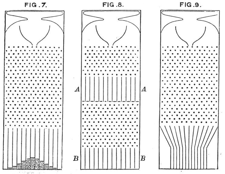
  • The name of the language comes from a physical device for visualizing probability distributions because that’s what it does.


I will likely do a whole series on Bean Machine later on this autumn, but for today let me just give you the brief overview should you not want to go through the paper. As the paper’s title says, Bean Machine is a Probabilistic Programming Language (PPL).

For a detailed introduction to PPLs you should read my “Fixing Random” series, where I show how we could greatly improve support for analysis of randomness in .NET by both adding types to the base class library and by adding language features to a language like C#.

If you don’t want to read that 40+ post introduction, here’s the TLDR.

We are all used to two basic kinds of programming: produce an effect and compute a result. The important thing to understand is that Bean Machine is firmly in the “compute a result” camp. In our PPL the goal of the programmer is to declaratively describe a model of how the world works, then input some observations of the real world in the context of the model, and have the program produce posterior distributions of what the real world is probably like, given those observations. It is a language for writing statistical model simulations.

A “hello world” example will probably help. Let’s revisit a scenario I first discussed in part 30 of Fixing Random: flipping a coin that comes from an unfair mint. That is, when you flip a coin from this mint, you do not necessarily have a 50-50 chance of getting heads vs tails. However, we do know that when we mint a coin, the distribution of fairness looks like this:

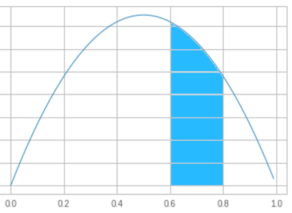
Fairness is along the x axis; 0.0 means “always tails”, 1.0 means “always heads”. The probability of getting a coin of a particular fairness is proportional to the area under the graph. In the graph above I highlighted the area between 0.6 and 0.8; the blue area is about 25% of the total area under the curve, so we have a 25% chance that a coin will be between 0.6 and 0.8 fair.

Similarly, the area between 0.4 and 0.6 is about 30% of the total area, so we have a 30% chance of getting a coin whose fairness is between 0.4 and 0.6. You see how this goes I’m sure.

Suppose we mint a coin; we do not know its true fairness, just the distribution of fairness above. We flip the coin 100 times, and we get 72 heads, 28 tails. What is the most probable fairness of the coin?

Well, obviously the most probable fairness of a coin that comes up heads 72 times out of 100 is 0.72, right?

Well, no, not necessarily right. Why? Because the prior probability that we got a coin that is between 0.0 and 0.6 is rather a lot higher than the prior probability that we got a coin between 0.6 and 1.0. It is possible by sheer luck to get 72 heads out of 100 with a coin between 0.0 and 0.6 fairness, and those coins are more likely overall.


Aside: If that is not clear, try thinking about an easier problem that I discussed in my earlier series. You have 999 fair coins and one double-headed coin. You pick a coin at random, flip it ten times and get ten heads in a row. What is the most likely fairness, 0.5 or 1.0? Put another way: what is the probability that you got the double-headed coin? Obviously it is not 0.1%, the prior, but nor is it 100%; you could have gotten ten heads in a row just by luck with a fair coin. What is the true posterior probability of having chosen the double-headed coin given these observations?


What we have to do here is balance between two competing facts. First, the fact that we’ve observed some coin flips that are most consistent with 0.72 fairness, and second, the fact that the coin could easily have a smaller (or larger!) fairness and we just got 72 heads by luck. The math to do that balancing act to work out the true distribution of possible fairness is by no means obvious.

What we want to do is use a PPL like Bean Machine to answer this question for us, so let’s build a model!

The code will probably look very familiar, and that’s because Bean Machine is a declarative language based on Python; all Bean Machine programs are also legal Python programs. We begin by saying what our “random variables” are.


Aside: Statisticians use “variable” in a way very different than computer programmers, so do not be fooled here by your intuition. By “random variable” we mean that we have a distribution of possible random values; a representation of any single one of those values drawn from a distribution is a “random variable”. 


To represent random variables we declare a function that returns a pytorch distribution object for the distribution from which the random variable has been drawn. The curve above is represented by the function beta(2, 2), and we have a constructor for an object that represents that distribution in the pytorch library that we’re using, so:

@random_variable
def coin():
  return Beta(2.0, 2.0)

Easy as that. Every usage in the program of coin() is logically a single random variable; that random variable is a coin fairness that was generated by sampling it from the beta(2, 2) distribution graphed above.


Aside: The code might seem a little weird, but remember we do these sorts of shenanigans all the time in C#. In C# we might have a method that looks like it returns an int, but the return type is Task<int>; we might have a method that yield returns a double, but the return type is IEnumerable<double>. This is very similar; the method looks like it is returning a distribution of fairnesses, but logically we treat it like a specific fairness drawn from that distribution.


What do we then do? We flip a coin 100 times. We therefore need a random variable for each of those coin flips:

@random_variable
def flip(i):
  return Bernoulli(coin())

Let’s break that down. Each call flip(0), flip(1), and so on on, are distinct random variables; they are outcomes of a Bernoulli process — the “flip a coin” process — where the fairness of the coin is given by the single random variable coin(). But every call to flip(0) is logically the same specific coin flip, no matter how many times it appears in the program.

For the purposes of this exercise I generated a coin and simulated 100 coin tosses to simulate our observations of the real world. I got 72 heads. Because I can peek behind the curtain for the purposes of this test, I can tell you that the coin’s true fairness was 0.75, but of course in a real-world scenario we would not know that. (And of course it is perfectly plausible to get 72 heads on 100 coin flips with a 0.75 fair coin.)

We need to say what our observations are.  The Bernoulli distribution in pytorch produces a 1.0 tensor for “heads” and a 0.0 tensor for “tails”. Our observations are represented as a dictionary mapping from random variables to observed values.

heads = tensor(1.0)
tails = tensor(0.0)
observations = {
  flip(0) : heads,
  flip(1) : tails,
  ...  and so on, 100 times with 72 heads, 28 tails.
}

Finally, we have to tell Bean Machine what to infer. We want to know the posterior probability of fairness of the coin, so we make a list of the random variables we care to infer posteriors on; there is only one in this case.

inferences = [ coin() ]
posteriors = infer(observations, inferences)
fairness = posteriors[coin()]

and we get an object representing samples from the posterior fairness of the coin given these observations. (I’ve simplified the call site to the inference method slightly here for clarity; it takes more arguments to control the details of the inference process.)

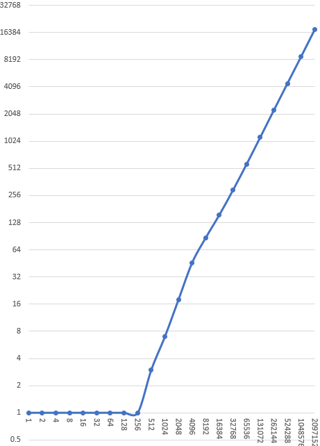
The “fairness” object that is handed back is the result of efficiently simulating the possible worlds that get you to the observed heads and tails; we then have methods that allow you to graph the results of those simulations using standard graphing packages:

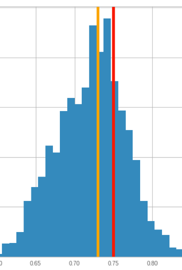
The orange marker is our original guess of observed fairness: 0.72. The red marker is the actual fairness of the coin used to generate the observations, 0.75. The blue histogram shows the results of 1000 simulations; the vast majority of simulations that produced those 72 heads had a fairness between 0.6 and 0.8, even though only 25% of the coins produced by the mint are in that range.  As we would hope, both the orange and red markers are near the peak of the histogram.

So yes, 0.72 is close to the most likely fairness, but we also see here that a great many other fairnesses are possible, and moreover, we clearly see how likely they are compared to 0.72. For example, 0.65 is also pretty likely, and it is much more likely than, say, 0.85. This should make sense, since the prior distribution was that fairnesses closer to 0.5 are more likely than those farther away; there’s more “bulk” to the histogram to the left than the right: that is the influence of the prior on the posterior!

Of course because we only did 1000 simulations there is some noise; if we did more simulations we would get a smoother result and a clear, single peak. But this is a pretty good estimate for a Python program with six lines of model code that only takes a few seconds to run.


Why do we care about coin flips? Obviously we don’t care about solving coin flip problems for their own sake. Rather, there are a huge number of real-world problems that can be modeled as coin flips where the “mint” produces unfair coins and we know the distribution of coins that come from that mint:

  • A factory produces routers that have some “reliability”; each packet that passes through each router in a network “flips a coin” with that reliability; heads, the packet gets delivered correctly, tails it does not. Given some observations from a real data center, which is the router that is most likely to be the broken one? I described this model in my Fixing Random series.
  • A human reviewer classifies photos as either “a funny cat picture” or “not a funny cat picture”. We have a source of photos — our “mint” — that produces pictures with some probability of them being a funny cat photo, and we have human reviewers each with some individual probability of making a mistake in classification. Given a photo and ten classifications from ten reviewers, what is the probability that it is a funny cat photo? Again, each of these actions can be modeled as a coin flip.
  • A new user is either a real person or a hostile robot, with some probability. The new user sends a friend request to you; you either accept it or reject it based on your personal likelihood of accepting friend requests. Each one of these actions can be modeled as a coin flip; given some observations of all those “flips”, what is the posterior probability that the account is a hostile robot?

And so on; there are a huge number of real-world problems we can solve just with modeling coin flips, and Bean Machine does a lot more than just coin flip models!


I know that was rather a lot to absorb, but it is not every day you get a whole new programming language to explain! In future episodes I’ll talk more about how Bean Machine works behind the scenes, how we traded off between declarative and imperative style, and that sort of thing. It’s been a fascinating journey so far and I can’t hardly wait to share it.


Life, part 35

Last time we implemented what looked like Gosper’s algorithm and got a disappointing result; though the quadtree data structure is elegant and the recursive algorithm is simple, and even though we memoize every operation, the time performance is on par with our original naive implementation, and the amount of space consumed by the memoizers is ginormous. But as I said last time, I missed a trick in my description of the algorithm, and that trick is the key to the whole thing. (Code for this episode is here.)

One reader pointed out that we could be doing a better job with the caching. Sure, that is absolutely true. There are lots of ways we could come up with a better cache mechanism than my hastily-constructed dictionary, and those would in fact lead to marginal performance gains. But I was looking for a win in the algorithm itself, not in the details of the cache.

A few readers made the astute observation that the number of recursions — nine — was higher than necessary. The algorithm I gave was:

  • We are given an n-quad and wish to step the center (n-1)-quad.
  • We make nine unstepped (n-1)-quads and step each of them to get nine stepped (n-2)-quads
  • We reform those nine (n-2)-quads into four stepped (n-1)-quads, take the centers of each, and that’s our stepped (n-1) quad.

But we have all the information we need in the original n-quad to extract four unstepped (n-1)-quads. We then could step each of those to get four center stepped (n-2)-quads, and we can reform those into the desired (n-1)-quad.

Extracting those four unstepped (n-1)-quads is a fair amount of work, but there is an argument to be made that it might be worth the extra work in order to go from nine recursions to four. I didn’t try it, but a reader did and reports back that it turns out this is not a performance win. Regardless though, this wasn’t the win I was looking for.

Let’s go through the derivation one more time, and derive Gosper’s algorithm for real.

We still have our base case: we can take any 2-quad and get the center 1-quad stepped one tick forward. Suppose once again we are trying to step the outer green 3-quad forward; we step each of its component green 2-quads forward one tick to get these four blue 1-quads:

We then extract the north, south, east, west and center 2-quads from the 3-quad and step each of those forwards one tick, and that gives us these nine blue 1-quads, each one step in the future:


We then form four 2-quads from those nine 1-quads; here we are looking at the northwest 2-quad and its center 1-quad:

The light blue 2-quad and its dark blue 1-quad center are both one tick ahead of the outer green 3-quad. This is where we missed our trick.

We have the light blue 2-quad, and it is one tick ahead of the green 3-quad. We want to get its center 1-quad. What if we got its center 1-quad stepped one tick ahead? We know we can do it! It’s a 2-quad and we can get the center 1-quad of any 2-quad stepped one tick ahead. We can make the innermost dark blue quad stepped two ticks ahead. We repeat that operation four times and we have enough information to construct…

…the center 2-quad stepped two ticks ahead, not one.

Now let’s do the same reasoning for a 4-quad.

We step its nine component 3-quads forwards two ticks, because as we just saw, we can do that for a 3-quad. We then compose those nine 2-quads into four 3-quads, step each of those forward two ticks, again because we can, and construct the center 3-quad stepped four ticks ahead.

And now let’s do the same reasoning for an n-quad… you see where this is going I’m sure.

This is the astonishing power of Gosper’s algorithm. Given an n-quad, we can step forward its center (n-1)-quad by 2n-2 ticks for any n>=2.

Want to know the state of the board a million ticks in the future? Embiggen the board until it is a 22-quad — we know that operation is cheap and easy — and you can get the center 21-quad stepped forwards by 220 ticks using this algorithm. A billion ticks? Embiggen it to a 32-quad, step it forward 230 ticks.

We showed last time an algorithm for stepping an n-quad forward by one tick; here we’ve sketched an algorithm for stepping an n-quad forward by 2n-2 ticks. What would be really nice from a user-interface perspective is if we had a hybrid algorithm that can step an n-quad forward by 2k ticks for any k between 0 and n-2.

You may recall that many episodes ago I added an exponential “speed factor” where the factor is the log2 of the number of ticks to step. We can now write an implementation of Gosper’s algorithm for real this time that takes a speed factor. Rather than try to explain it further, let’s just look at the code.

private static Quad UnmemoizedStep((Quad q, int speed) args)
{
  Quad q = args.q;
  int speed = args.speed;

  Debug.Assert(q.Level >= 2);
  Debug.Assert(speed >= 0);
  Debug.Assert(speed <= q.Level - 2);

  Quad r;
  if (q.IsEmpty)
    r = Quad.Empty(q.Level - 1);
  else if (speed == 0 && q.Level == 2)
    r = StepBaseCase(q);
  else
  {
    // The recursion requires that the new speed be not
    // greater than the new level minus two. Decrease speed
    // only if necessary.
    int nineSpeed = (speed == q.Level - 2) ? speed - 1 : speed;
    Quad q9nw = Step(q.NW, nineSpeed);
    Quad q9n = Step(q.N, nineSpeed);
    Quad q9ne = Step(q.NE, nineSpeed);
    Quad q9w = Step(q.W, nineSpeed);
    Quad q9c = Step(q.Center, nineSpeed);
    Quad q9e = Step(q.E, nineSpeed);
    Quad q9sw = Step(q.SW, nineSpeed);
    Quad q9s = Step(q.S, nineSpeed);
    Quad q9se = Step(q.SE, nineSpeed);
    Quad q4nw = Make(q9nw, q9n, q9c, q9w);
    Quad q4ne = Make(q9n, q9ne, q9e, q9c);
    Quad q4se = Make(q9c, q9e, q9se, q9s);
    Quad q4sw = Make(q9w, q9c, q9s, q9sw);

    // If we are asked to step forwards at speed (level - 2), 
    // then we know that the four quads we just made are stepped 
    // forwards at (level - 3). If we step each of those forwards at 
    // (level - 3) also, then we have the center stepped forward at 
    // (level - 2), as desired.
    //
    // If we are asked to step forwards at less than speed (level - 2)
    // then we know the four quads we just made are already stepped
    // that amount, so just take their centers.

    if (speed == q.Level - 2)
    {  
      Quad rnw = Step(q4nw, speed - 1);
      Quad rne = Step(q4ne, speed - 1);
      Quad rse = Step(q4se, speed - 1);
      Quad rsw = Step(q4sw, speed - 1);
      r = Make(rnw, rne, rse, rsw);
    }
    else
    {
      Quad rnw = q4nw.Center;
      Quad rne = q4ne.Center;
      Quad rse = q4se.Center;
      Quad rsw = q4sw.Center;
      r = Make(rnw, rne, rse, rsw);
    }
  }
  Debug.Assert(q.Level == r.Level + 1);
  return r;
}

As I’m sure you’ve guessed, yes, we’re going to memoize this too! This power has not come for free; we are now doing worst case 13 recursions per non-base call, which means that we could be doing worst case 13n-3 base case calls in order to step forwards 2n-2 ticks, and that’s a lot of base case calls. How on earth is this ever going to work?

Again, because (1) we are automatically skipping empty space of every size; if we have an empty 10-quad that we’re trying to step forwards 256 ticks, we immediately return an empty 9-quad, and (2) thanks to memoization every time we encounter a problem we’ve encountered before, we just hand back the solution. The nature of Life is that you frequently encounter portions of boards that you’ve seen before because most of a board is stable most of the time. We hope.

That’s the core of Gosper’s algorithm, finally. (Sorry it took 35 episodes to get there, but it was a fun journey!) Let’s now integrate that into our existing infrastructure; I’ll omit the memoization and cache management because it’s pretty much the same as we’ve seen already.

The first thing to note is that we can finally get rid of this little loop:

public void Step(int speed)
{
  for (int i = 0; i < 1L << speed; i += 1)
    Step();
}

Rather than implementing Step(speed) in terms of Step(), we’ll go the other way:

public void Step()
{
  Step(0);
}

public void Step(int speed)
{
  // Cache management omitted
  const int MaxSpeed = MaxLevel - 2;
  Debug.Assert(speed >= 0);
  Debug.Assert(speed <= MaxSpeed);

The embiggening logic needs to be a little more aggressive. This implementation is probably more aggressive than we need it to be, but remember, empty space is essentially free both in space and processing time.

  Quad current = cells;
  if (!current.HasAllEmptyEdges)
    current = current.Embiggen().Embiggen();
  else if (!current.Center.HasAllEmptyEdges)
    current = current.Embiggen();
  while (current.Level < speed + 2)
    current = current.Embiggen();

  Quad next = Step(current, speed);
  cells = next.Embiggen();
  generation += 1L << speed;
  // Cache reset logic omitted
}

Now how are we going to perf test this thing? We already know that calculating 5000 individual generations of “acorn” with Gosper’s algorithm will be as slow as the original naïve version. What happens if for our performance test we set up acorn and then call Step(13)? That will step it forwards 8196 ticks:

Algorithm           time(ms) size  Mcells/s 
Naïve (Optimized):   4000     8      82     
Abrash (Original)     550     8     596     
Stafford              180     8    1820     
QuickLife              65    20      ?      
Gosper, sp 0 * 5000  3700    60      ?
Gosper, sp 13 * 1     820    60      ?

Better, but still not as good as any of our improvements over the naïve algorithm, and 13x slower than QuickLife.

So this is all very interesting, but what’s the big deal?

Do you remember the asymptotic time performance of Hensel’s QuickLife? It was O(changes); that is, the cost of computing one tick forwards is proportional to the number of changed cells on that tick. Moreover, period-two oscillators were essentially seen as not changing, which is a huge win.

We know that the long-term behaviour of acorn is that shortly after 5000 ticks in, we have only a handful of gliders going off to infinity and all the rest of the living cells are either still Lifes or period-two oscillators that from QuickLife’s perspective, might as well be still Lifes. So in the long run, the only changes that QuickLife has to process are the few dozens of cells changed for each glider; everything else gets moved into the “stable” bucket.

Since in the long run QuickLife is processing the same number of changes per tick, we would expect that the total time taken to run n ticks of acorn with QuickLife should grow linearly. Let’s actually try it out to make sure. I’m going to run one ticks of acorn with QuickLife, then reset, then run two ticks , then reset, then run four ticks, reset, eight ticks, and so on, measuring the time for each, up to 221 =~ 2.1 million ticks.

Here is a graph of the results; milliseconds on the y axis, ticks on the x axis, log-log scale. Lower is faster.


Obviously the leftmost portion of the graph is wrong; anything less than 256 ticks takes less than 1 millisecond but I haven’t instrumented my implementation to measure sub-millisecond timings because I don’t care about those. I’ve just marked all of them as taking one millisecond.

Once we’re over a millisecond, you can see that QuickLife’s time to compute some number of ticks grows linearly; it’s about 8 microseconds per tick, which is pretty good. You can also see that the line changes slope slightly once we get to the point where it is only the gliders on the active list; the slope gets shallower, indicating that we’re taking less time for each tick.

Now let’s do the same with Gosper’s algorithm; of course we will make sure to reset the caches between every run! Otherwise we would be unfairly crediting speed improvements in later runs to cached work that was done in earlier runs.

Hensel’s QuickLife in blue, Gosper’s HashLife in orange:

Holy goodness! 

The left hand side of the graph shows that Gosper’s algorithm is consistently around 16x slower than QuickLife in the “chaos” part of acorn’s evolution, right up to the point where we end up in the “steady state” of just still Lifes, period-two oscillators and gliders. The right hand side of the graph shows that once we are past that point, Gosper’s algorithm becomes O(1), not O(changes).

In fact this trend continues. We can compute a million, a billion, a trillion, a quadrillion ticks of acorn in around 800ms. And we can embiggen the board to accurately track the positions of those gliders even when they are a quadrillion cells away from the center.

What is the takeaway here? The whole point of this series is: you can take advantage of characteristics of your problem space to drive performance improvements. But what we’ve just dramatically seen here is that this maxim is not sufficient. You’ve also got to think about specific problems that you are solving.

Let’s compare and contrast. Hensel’s QuickLife algorithm excels when:

  • All cells of interest fit into a 20-quad
  • There is a relatively small number of living cells (because memory burden grows as O(living)
  • You are making a small number of steps at a time
  • Living cells are mostly still Lifes or period-two oscillators; the number of “active” Quad4s is relatively small

Gosper’s HashLife algorithm excels when:

  • Boards must be of unlimited size
  • Regularity in space — whether empty space or not — allows large regions to be deduplicated
  • You are making a large number of steps at a time
  • Regularity in time allows for big wins by caching and re-using steps we’ve seen already.
  • You’ve got a lot of memory! Because the caches are going to get big no matter what you do.

That’s why Gosper’s algorithm is so slow if you run in on the first few thousand generations of acorn; that evolution is very chaotic and so there are a lot of novel computations to do and comparatively less re-use. Once we’re past the chaotic period, things become very regular in both time and space, and we transition to a constant-time performance.


That is the last algorithm I’m going to present but I have one more thing to discuss in this series.

Next time on FAIC: we will finally answer the question I have been teasing all this time: are there patterns that grow quadratically? And how might our two best algorithms handle such scenarios?


Life, part 34

All right, we have our quad data structure, we know how to get and set individual elements, and we know how to display it. We’ve deduplicated it using memoization. How do we step it forward one tick? (Code for this episode is here.)

Remember a few episodes ago when we were discussing QuickLife and noted that if you have a 2-quad in hand, like these green ones, you can get the state of the blue 1-quad one tick ahead? And in fact we effectively memoized that solution by simply precomputing all 65536 cases.

The QuickLife algorithm memoized only the 2-quad-to-center-1-quad step algorithm; we’re going to do the same thing but with even more memoization. We have a recursively defined quad data structure, so it makes sense that the step algorithm will be recursive. We will use 2-quad-to-1-quad as our base case.

For the last time in this series, let’s write the Life rule:

private static Quad Rule(Quad q, int count)
{
  if (count == 2) return q;
  if (count == 3) return Alive;
  return Dead;
}

We’ll get all sixteen cells in the 2-quad as numbers:

private static Quad StepBaseCase(Quad q)
{
  Debug.Assert(q.Level == 2);
  int b00 = (q.NW.NW == Dead) ? 0 : 1;
  ... 15 more omitted ...

and count the neighbours of the center 1-quad:

  int n11 = b00 + b01 + b02 + b10 + b12 + b20 + b21 + b22;
  int n12 = b01 + b02 + b03 + b11 + b13 + b21 + b22 + b23;
  int n21 = b11 + b12 + b13 + b21 + b23 + b31 + b32 + b33;
  int n22 = b10 + b11 + b12 + b20 + b22 + b30 + b31 + b32;
  return Make(
    Rule(q.NW.SE, n11),
    Rule(q.NE.SW, n12),
    Rule(q.SE.NW, n21),
    Rule(q.SW.NE, n22));
}

We’ve seen this half a dozen times before. The interesting bit comes in the recursive step. The key insight is: for any n>=2, if you have an n-quad in hand, you can compute the (n-1) quad in the center, one tick ahead.

How? We’re going to use almost the same technique that we used in QuickLife. Remember in QuickLife the key was observing that if we had nine Quad2s in the old generation, we could compute a Quad3 in the new generation with sixteen steps on component Quad2s. The trick here is almost the same. Let’s draw some diagrams.

Suppose we have the 3-quad from the image above. We compute the next generation of its four component 2-quads; the green quads are current, the blue are stepped one ahead.

We can use a similar trick as we used with QuickLife to get the north, south, east, west and center 2-quads of this 3-quad, and move each of them ahead one step to get five more 1-quads. I’ll draw the original 3-quad in light green, and we can extract component 2-quads from it that I’ll draw in dark green. We then move each of those one step ahead to get the blue 1-quads.

That gives us this information:

We then make four 2-quads from those nine: and extract the center 1-quad from each using the Center function (source code below). I’ll just show the northwest corner; you’ll see how this goes. We make the light blue 2-quad out of four of the blue 1-quads, and then the center 1-quad of that thing is:

We do that four times and from those 1-quads we construct the center 2-quad moved one step ahead:

Summing up the story so far:

  • We can take a 2-quad forward one tick to make a 1-quad with our base case.
  • We’ve just seen here that we can use that fact to take a 3-quad forward one tick to make a 2-quad stepped forward one tick.
  • But nothing we did in the previous set of steps depended on having a 3-quad specifically. Assume that for some n >= 2 we can move an n-quad forward one tick to make an (n-1) quad; we have above an algorithm where we use that assumption and can move an (n+1)-quad forward to get an n-quad.

That is, we can move a 2-quad forward with our base case; moving a 3-quad forward requires the ability to move a 2-quad forward. Moving a 4-quad forward requires the ability to move a 3-quad forward, and so on.

As I’ve said many times on this blog, every recursive algorithm is basically the same. If we’re in the base case, solve the problem directly. If we’re not in the base case, break up the problem into finitely many smaller problems, solve each, and use the solutions to solve the larger problem.

Let’s write the code to move any n-quad for n >= 2 forward one tick.

We’ll need some helper methods that extract the five needed sub-quads, but those are easily added to Quad. (Of course these helpers are only valid when called on a 2-quad or larger.)

public Quad Center => Make(NW.SE, NE.SW, SE.NW, SW.NE);
public Quad N => Make(NW.NE, NE.NW, NE.SW, NW.SE);
public Quad E => Make(NE.SW, NE.SE, SE.NE, SE.NW);
public Quad S => Make(SW.NE, SE.NW, SE.SW, SW.SE);
public Quad W => Make(NW.SW, NW.SE, SW.NE, SW.NW);

And then I’ll make a static method that takes a Quad and returns the center stepped forward one tick. (Why not an instance method on Quad? We will see in a moment.)

private static Quad Step(Quad q)
{
  Debug.Assert(q.Level >= 2);
  Quad r;
  if (q.IsEmpty)
    r = Empty(q.Level - 1);
  else if (q.Level == 2)
    r = StepBaseCase(q);
  else
  {
    Quad q9nw = Step(q.NW);
    Quad q9n = Step(q.N);
    Quad q9ne = Step(q.NE);
    Quad q9w = Step(q.W);
    Quad q9c = Step(q.Center);
    Quad q9e = Step(q.E);
    Quad q9sw = Step(q.SW);
    Quad q9s = Step(q.S);
    Quad q9se = Step(q.SE);
    Quad q4nw = Make(q9nw, q9n, q9c, q9w);
    Quad q4ne = Make(q9n, q9ne, q9e, q9c);
    Quad q4se = Make(q9c, q9e, q9se, q9s);
    Quad q4sw = Make(q9w, q9c, q9s, q9sw);
    Quad rnw = q4nw.Center;
    Quad rne = q4ne.Center;
    Quad rse = q4se.Center;
    Quad rsw = q4sw.Center;
    r = Make(rnw, rne, rse, rsw);
  }
  Debug.Assert(q.Level == r.Level + 1);
  return r;
}

Well that was easy! We just do nine recursions and then reorganize the resulting nine one-tick-forward quads until we get the information we want, and return it. (I added a little easy out for the empty case, though strictly speaking that is not necessary.)

There are probably three things on your mind right now.

  • If we get a full quad-size smaller every time we step, we’re going to get down to a very small board very quickly!
  • QuickLife memoized the step-the-center-of-a-2-quad operation. Why aren’t we doing the same thing here?
  • Nine recursions is a lot; isn’t this going to blow up performance? Suppose we have an 8-quad; we do nine recursions on 7-quads, but each of those does nine recursions on 6-quads, and so on down to 3-quads. It looks like we are doing 9n-2 calls to the base case when stepping an n-quad forward one tick.

First things first.

When do we not care if we’re shrinking an n-quad down to an (n-1)-quad on step? When all living cells in the n-quad are already in the center (n-1)-quad. But that condition is easy to achieve! Let’s actually write our public step method, not just the helper that steps a quad. And heck, let’s make sure that we have more than enough empty space. Remember, empty space is super cheap. 

sealed class Gosper : ILife, IDrawScale, IReport
{
  private Quad cells;
  private long generation;
  ...
  public void Step()
  {
    Quad current = cells;

Make cells bigger until there are two “levels” of empty cells surrounding the center. (We showed Embiggen last time.) That way we are definitely not throwing away any living cells when we get a next state that is one size smaller:

    if (!current.HasAllEmptyEdges)
      current = current.Embiggen().Embiggen();
    else if (!current.Center.HasAllEmptyEdges)
      current = current.Embiggen();
    Quad next = Step(current);

We’ve stepped, so next is one size smaller than current. Might as well make it bigger too; that’s one fewer thing to deal with next time. Again, empty space is cheap.

  cells = next.Embiggen();
  generation += 1;
}

HasAllEmptyEdges is an easy helper method of Quad:

public bool HasAllEmptyEdges => 
  NW.NW.IsEmpty &&
  NW.NE.IsEmpty &&
  NE.NW.IsEmpty &&
  NE.NE.IsEmpty &&
  NE.SE.IsEmpty &&
  SE.NE.IsEmpty &&
  SE.SE.IsEmpty &&
  SE.SW.IsEmpty &&
  SW.SE.IsEmpty &&
  SW.SW.IsEmpty &&
  SW.NW.IsEmpty &&
  NW.SW.IsEmpty;

That was an easy problem to knock down. Second problem: QuickLife memoized the 2-quad-to-1-quad step algorithm and got a big win; shouldn’t we do the same thing?

Sure, we have a memoizer, we can do so easily. But… what about our third problem? We have a recursive step that is creating exponentially more work as the quad gets larger as it traverses our deduplicated tree structure.

Hmm.

It is recursing on a deduplicated structure, which means it is probably going to encounter the same problems several times. If we move a 3-quad forward one step to get a 2-quad, we’re going to get the same answer the second time we do the same operation on the same 3-quad. If we move a 4-quad forward one step to get a 3-quad, we will get the same answer the second time we do it. And so on. Let’s just memoize everything.

We’ll rename Step to UnmemoizedStep, create a third memoizer, and replace Step with:

private static Quad Step(Quad q) => 
  CacheManager.StepMemoizer.MemoizedFunc(q);

And now we have solved our second and third problems with one stroke.

Let’s run it! We’ll do our standard performance test of 5000 generations of acorn:

Algorithm           time(ms) size  Mcells/s 
Naïve (Optimized):   4000     8      82     
Abrash (Original)     550     8     596     
Stafford              180     8    1820     
QuickLife              65    20      ?      
Gosper v1            3700    60      ?

Oof.

It’s slow! Not as slow as the original naïve implementation, but just about.

Hmm.

That’s the time performance; what’s the memory performance? There’s a saying I’ve used many times; I first heard it from Raymond Chen but I don’t know if he coined it or was quoting someone else. “A cache without an expiration policy is called a memory leak”. Memory leaks can cause speed problems as well as memory problems because they increase burden on the garbage collector, which can slow down the whole system. Also, dictionaries are in theory O(1) access — that is, access time is the same no matter how big the cache gets — but theory and practice are often different as the dictionaries get very large.

How much memory are we using in this thing? The “empty” memoizer never has more than 61 entries, so we can ignore it. I did some instrumentation of the “make” and “step” caches; after 5000 generations of acorn:

  • the step and make caches both have millions of entries
  • half the entries were never read at all, only written
  • 97% of the entries were read fewer than twenty times
  • the top twenty most-read entries account for 40% of the total reads

This validates our initial assumption that there is a huge amount of regularity; the “unusual” situations recur a couple dozen times tops, and we spend most of our time looking at the same configurations over and over again.

This all suggests that we could benefit from an expiration policy. There are two things to consider: what to throw away, and when to throw it away. First things first:

  • An LRU cache seems plausible; that is, when you think it is time to take stuff out of the cache, take out some fraction of the stuff that has been Least Recently Used. However LRU caches involve making extra data structures to keep track of when something has been used; we do extra work on each step, and it seems like that might have a performance impact given how often these caches are hit.
  • The easiest policy is: throw it all away! Those 20 entries that make up 40% of the hits will be very quickly added back to the cache.

Let’s try the latter because it’s simple. Now, we cannot just throw it all away because we must maintain the invariant that Make agrees with Empty; that is, when we call Make with four empty n-quads and when we call Empty(n+1) we must get the same object out. But if we throw away the “make” cache and then re-seed it with the contents of the “empty” cache — which is only 61 entries, that’s easy — then we maintain that invariant.

When to throw it away? What we definitely do not want to happen is end up in a situation where we are throwing away stuff too often. We can make a very simple dynamically-tuned cache with this policy:

  • Set an initial cache size bound. 100K entries, 1M entries, whatever.
  • Every thousand generations, check to see if we’ve exceeded the cache size bound. If not, we’re done.
  • We’ve exceeded the bound. Throw away the caches, do a single step, and re-examine the cache size; this tells us the cache burden of doing one tick.
  • The new cache size bound is the larger of the current bound and twice the one-tick burden. That way if necessary the size bound gradually gets larger so we do less frequent cache resetting.

The code is straightforward; at the start of Step:

bool resetMaxCache = false;
if ((generation & 0x3ff) == 0)
{
  int cacheSize = CacheManager.MakeQuadMemoizer.Count + 
    CacheManager.StepMemoizer.Count;
  if (cacheSize > maxCache)
  {
    resetMaxCache = true;
    ResetCaches();
  }
}

“ResetCaches” throws away the step cache and resets the make cache to agree with the empty cache; I won’t bother to show it. At the end of Step:

if (resetMaxCache)
{
  int cacheSize = CacheManager.MakeQuadMemoizer.Count + 
    CacheManager.StepMemoizer.Count;
  maxCache = Max(maxCache, cacheSize * 2);
}

All right, let’s run it again!

Algorithm           time(ms) size  Mcells/s 
Naïve (Optimized):   4000     8      82     
Abrash (Original)     550     8     596     
Stafford              180     8    1820     
QuickLife              65    20      ?      
Gosper v2            4100    60      ?

It’s worse. Heck, it is worse than the naive algorithm!

Sure, the top twenty cache entries account for 40% of the hits, and sure, 97% of the entries are hit fewer than twenty times. But the statistic that is relevant here that I omitted is: the top many hundreds of cache entries account for 50% of the hits. We don’t have to rebuild just the top twenty items in the cache to start getting a win from caching again. We take a small but relevant penalty every time we rebuild the caches.

Sigh.

We could keep on trying to improve the marginal performance by improving our mechanisms. We could try an LRU cache, or optimize the caches for reading those top twenty entries, or whatever. We might eke out some wins. But maybe instead we should take a step back and ask if there’s an algorithmic optimization that we missed.


Next time on FAIC: There is an algorithmic optimization that we missed. Can you spot it?

Installing windows

Episode 34 will be delayed again — sorry! — because once again the time I had set aside for writing this weekend got consumed by a real-world task that could not wait. (I will try for Thursday of this week.)

Some friends who are moving had a handyman failure; as is often the case when renovating a house to be sold, they have a set of build dependencies that required this window to be replaced in a hurry in order to not slip the schedule for other renovations, so I volunteered to take care of it.

Yuck.

Living in a 112 year old house myself, I am used to doing archaeological investigations of the strange decisions made by previous owners. This window, though obviously an old single-paned window, did not look like it was original to the 120-year-old house. It was the wrong size for the rough opening; the hinges looked more modern than turn-of-the-century, and so on.

Sure enough, when disassembled there was a gap behind the trim that was insulated with crumpled newspapers from 1957. Oddly enough they were Pittsburgh newspapers from different days; perhaps the owners of the house in 1957 moved from Pittsburgh, replaced a window, and insulated the gaps with the packing paper they moved with? It’s a mystery.

Having zero haircuts since quarantine began has done wonders for my hair.

New window in and trimmed — obviously the paint will need to be redone but that’s why the window had to go in before the painters arrived.

And the interior needs a little more drywalling and priming before it is ready for painting, but it is 1000000x better than before at least.

The neighbours in the blue house apparently asked my friends for my contact information as they also have a window that needs replacing. I am quite chuffed. I had my friends pass along that I only do windows as a favour, but I would be happy to design them a programming language for hire should they need one of those.

Next time: Gosper’s algorithm, finally!