One more time! Suppose we have our nominal distribution p that possibly has “black swans” and our helper distribution q which has the same support, but no black swans.

We wish to compute the expected value of f when applied to samples from p, and we’ve seen that we can estimate it by computing the expected value of g:

x => f(x) * p.Weight(x) / q.Weight(x)

applied to samples of q.

Unfortunately, the last two times on FAIC we saw that the result will be wrong by a constant factor; the constant factor is the quotient of the normalization constants of q and p.

It seems like we’re stuck; it can be expensive or difficult to determine the normalization factor for an arbitrary distribution. We’ve created infrastructure for building weighted distributions and computing posteriors and all sorts of fun stuff, and none of it assumes that weights are normalized so that the area under the PDF is 1.0.

But… we don’t need to know the normalization factors. We never did, and every time I said we did, I lied to you. Because I am devious.

What do we really need to know? We need to know the quotient of two normalization constants. That is less information than knowing two normalization constants, and maybe there is a cheap way to compute that fraction.

Well, let’s play around with computing fractions of weights; our intuition is: maybe the quotient of the normalization constants is the average of the quotients of the weights. So let’s make a function and call it h:

x => p.Weight(x) / q.Weight(x)

What is the expected value of h when applied to samples drawn from q?

Well, we know that it could be computed by:

Area(x => h(x) * q.Weight(x)) / Area(q.Weight)

But do the algebra: that’s equal to

Area(p.Weight) / Area(q.Weight)

Which is the inverse of the quantity that we need, so we can just divide by it instead of multiplying!

Here’s our logic:

• We can estimate the expected value of g on samples of  q by sampling.
• We can estimate the expected value of h on samples of q by sampling.
• The quotient of these two estimates is an estimate of the expected value of f on samples of p, which is what we’ve been after this whole time.

Whew!

Aside: I would be remiss if I did not point out that there is one additional restriction that we’ve got to put on helper distribution q : there must be no likely values of x in the support of q such that q.Weight(x) is tiny but p.Weight(x) is extremely large, because their quotient is then going to blow up huge if we happen to sample that value, and that’s going to wreck the average.

We can now actually implement some code that computes expected values using importance sampling and no quadrature. Let’s put the whole thing together, finally: (All the code can be found here.)

public static double ExpectedValueBySampling<T>(
    this IDistribution<T> d,
    Func<T, double> f,
    int samples = 1000) =>
  d.Samples().Take(samples).Select(f).Average();

public static double ExpectedValueByImportance(
    this IWeightedDistribution<double> p,
    Func<double, double> f,
    double qOverP,
    IWeightedDistribution<double> q,
    int n = 1000) =>
  qOverP * q.ExpectedValueBySampling(
    x => f(x) * p.Weight(x) / q.Weight(x), n);

public static double ExpectedValueByImportance(
  this IWeightedDistribution<double> p,
  Func<double, double> f,
  IWeightedDistribution<double> q,
  int n = 1000)
{
  var pOverQ = q.ExpectedValueBySampling(
    x => p.Weight(x) / q.Weight(x), n);
  return p.ExpectedValueByImportance(f, 1.0 / pOverQ, q, n);
}

Look at that; the signatures of the methods are longer than the method bodies! Basically there’s only four lines of code here. Obviously I’m omitting error handling and parameter checking and all that stuff that would be necessary in a robust implementation, but the point is: even though it took me six math-heavy episodes to justify why this is the correct code to write, actually writing the code to solve this problem is very straightforward.

Once we have that code, we can use importance sampling and never have to do any quadrature, even if we do not give the ratio of the two normalization constants:

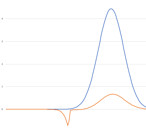
var p = Normal.Distribution(0.75, 0.09);
double f(double x) => Atan(1000 * (x – .45)) * 20 – 31.2;
var u = StandardContinuousUniform.Distribution;
var expected = p.ExpectedValueByImportance(f, u);

Summing up:

• If we have two distributions p and q with the same support…
• and a function f that we would like to evaluate on samples of p…
• and we want to estimate the average value of f …
• but p has “black swans” and q does not, then:
• we can still efficiently get an estimate by sampling q
• bonus: we can compute an estimate of the ratios of the normalization constants of p and q
• extra bonus: if we already know one of the normalization constants, we can compute an estimate of the other from the ratio.

Super; are we done?

In the last two episodes we pointed out that there are two problems: we don’t know the correction factor, and we don’t know how to pick a good q. We’ve only solved the first of those problems.

Next time on FAIC: We’ll dig into the problem of finding a good helper distribution q.

Last time on FAIC we deduced the idea behind the “importance sampling” technique for determining the average value of a function from double to double — call it  f — when it is applied to samples from a possibly-non-normalized weighted distribution of doubles — call it p.

Just for fun, I’m going to do the derivation all over again. I’ll again be using the technique “things equal to the same are equal to each other”, but this time we’re going to start from the other end. Let’s jump right in!

Again, for pedagogical purposes I’m going to consider only distributions with support from 0.0 to 1.0; we’ll eliminate that restriction when we can.

We discovered a while back that the expected value of f applied to samples of pis equal to the quotient of Area(x => f(x) * p.Weight(x) divided by ​​Area(x => p.Weight(x)). The latter term is the normalization constant for p, which we might not know.

Let’s take any weighted distribution q also with support from 0.0 to 1.0; it also might not be normalized.

We’re now going to do some manipulations to our expression that are obviously identities. We’ll start with the fact that

Area(x => f(x) * p.Weight(x))

obviously must be equal to:

Area(x => (f(x) * p.Weight(x) / q.Weight(x)) * q.Weight(x))

We’ve just divided and multiplied by the same quantity, so that is no change. And we’ve assumed that q has the same support as p, so the weight we’re dividing by is always non-zero.

Similarly,

Area(p.Weight)

must be equal to

(Area(q.Weight) * (Area(p.Weight) / Area(q.Weight)))

for the same reason.

So the quotient of these two quantities must also be equal to the expected value of f applied to samples from p; they’re the same quantities! Our original expression

Area(x => f(x) * p.Weight(x) /
 Area(x => p.Weight(x))

is equal to:

Area(x => (f(x) * p.Weight(x) / q.Weight(x)) * q.Weight(x)) / 
  (Area(q.Weight) * (Area(p.Weight) / Area(q.Weight)))

For any suitable q.

Let’s call that value exp_fp for “expected value of f on samples of p“. We’ve just written that value in two ways, one very straightforward, and one excessively complicated.

Unsurprisingly, my next question is: what is the expected value of function g

x => f(x) * p.Weight(x) / q.Weight(x)

over samples from q?

We know that it is estimated by this quotient of areas:

Area(x => g(x) * q.Weight(x)) /
Area(q.Weight)

The denominator is the normalization constant of q which we might not know.

Call that value exp_gq, for “expected value of g on samples of q”

What is the relationship between exp_gq and exp_fp?

Well, just look at the two expressions carefully; plainly they differ by no more than a constant factor. exp_fp is equal to exp_gq * Area(q.Weight) / Area(p.Weight)

And now we are right where we ended last time. Summing up:

• Once again, we have deduced that importance sampling works:
  • An estimate of the expected value of g applied to samples from q is proportional to the expected value of f applied to samples from p
  • the proportionality constant is exactly the quotient of the normalization constants of q and p
  • If q and p are known to be normalized, then that constant is 1.
• Once again, we can extend this result to q and p with any support
  • All we really need for an accurate estimate is that q have support in places where f(x) * p.Weight(x) has a lot of area.
  • But it is also nice if q has low weight in where that function has small area.
• Once again, we have two serious problems:
  • how do we find a good q?
  • we are required to know the normalization constants of both p and q, either of which might be hard to compute in general
• Once again, the previous statement contains a subtle error.
  • I’m so devious.
  • I asked what the error was in the previous episode as well, and there is already an answer in the comments to that episode, so beware of spoilers if you want to try to figure it out for yourself.

We are so close to success, but it seems to be just out of our grasp. It’s vexing!

Next time on FAIC: Amazingly, we’ll implement a version of this algorithm entirely based on sampling; we do not actually need to do the quadrature to compute the normalization factors!

Last time on FAIC we implemented a better technique for estimating the expected value of a function f applied to samples from a distribution p:

• Compute the total area (including negative areas) under the function x => f(x) * p.Weight(x)
• Compute the total area under x => p.Weight(x)
  • This is 1.0 for a normalized PDF, or the normalizing constant of a non-normalized PDF; if we already know it, we don’t have to compute it.
• The quotient of these areas is the expected value

Essentially our technique was to use quadrature to get an approximate numerical solution to an integral calculus problem.

However, we also noted that it seems like there might still be room for improvement, in two main areas:

• This technique only works when we have a good bound on the support of the distribution; for my contrived example I chose a “profit function” and a distribution where I said that I was only interested in the region from 0.0 to 1.0.
• Our initial intuition that implementing an estimate of “average of many samples” by, you know, averaging many samples, seems like it was on the right track; can we get back there?

In this episode I’m going to stick to the restriction to distributions with support over 0.0 to 1.0 for pedagogic reasons, but our aim is to find a technique that gets us back to sampling over arbitrary distributions.

The argument that I’m going to make here (several times!) is: two things that are both equal to the same third thing are also equal to each other.

Recall that we arrived at our quadrature implementation by estimating that our continuous distribution’s expected value is close to the expected value of a very similar discrete distribution. I’m going to make my argument a little bit more general here by removing the assumption that p is a normalized distribution. That means that we’ll need to know the normalizing factor np, which as we’ve noted is Area(p.Weight).

We said that we could estimate the expected value like this:

• Imagine that we create a 1000 sided “unfair die” discrete distribution.
• Each side corresponds to a 0.001 wide slice from the range 0.0 to 1.0; let’s say that we have a variable x that takes on values 0.000, 0.001, 0.002, and so on, corresponding to the 1000 sides.
• The weight of each side is the probability of choosing this slice: p.Weight(x) / 1000 / np
• The value of each side is the “profit function” f(x)
• The expected value of “rolling this die” is the sum of (value times weight): the sum of f(x) * (p.Weight(x) / 1000 / np)over our thousand values of x

Here’s the trick:

• Consider the standard continuous uniform distribution u. That’s a perfectly good distribution with support 0.0 to 1.0.
• Consider the function w(x) which is x => f(x) * p.Weight(x) / np.  That’s a perfectly good function from double to double.
• Question: What is an estimate of the expected value of w over samples from u?

We can use the same technique:

• Imagine we create a 1000-sided “unfair die” discrete distribution
• x is as before
• The weight of each side is the probability of choosing that slice, but since this is a uniform distribution, every weight is the same — so, turns out, it is not an unfair die! The weight of each side is 0.001.
•  The value of each side is our function w(x)
• The expected value of rolling this die is the sum of (value times weight): the sum of (f(x) * p.Weight(x) / np) * 0.001 over our thousand values of x

But compare those two expressions; we are computing exactly the same sum both times. These two expected values must be the same value.

Things equal to the same are equal to each other, which implies this conclusion:

If we can compute an estimate of the expected value of w applied to samples from u by any technique then we have also computed an estimate of the expected value of f applied to samples from p.

Why is this important?

The problem with the naïve algorithm in our original case was that there was a “black swan” — a region of large (negative) area that is sampled only one time in 1400 samples. But that region is sampled one time in about 14 samples when we sample from a uniform distribution, so we will get a much better and more consistent estimate of the expected value if we use the naïve technique over the uniform distribution.

In order to get 100x times as many samples in the black swan region, we do not have to do 100x times as many samples overall. We can just sample from a helper distribution that targets that important region more often.

Let’s try it! (Code can be found here.)

In order to not get confused here, I’m going to rename some of our methods so that they’re not all called ExpectedValue. The one that just takes any distribution and averages a bunch of samples is now ExpectedValueBySampling and the one that computes two areas and takes their quotient is ExpectedValueByQuadrature.

var p = Normal.Distribution(0.75, 0.09);
double f(double x) => Atan(1000 * (x – .45)) * 20 – 31.2;
var u = StandardContinuousUniform.Distribution;
double np = 1.0; // p is normalized
double w(double x) => f(x) * p.Weight(x) / np;
for (int i = 0; i < 100; ++i)
  Console.WriteLine($”{u.ExpectedValueBySampling(w):0.###}“);

Remember, the correct answer that we computed by quadrature is 0.113. When sampling p directly we got values ranging from 0.7 to 0.14. But now we get:

0.114, 0.109, 0.109, 0.118, 0.111, 0.107, 0.113, 0.112, ...

So much better!

This is awesome, but wait, it gets more awesome. What is so special about the uniform distribution? Nothing, that’s what. I’m going to do this argument one more time:

Suppose I have distribution q, any distribution whatsoever, so long as its support is the same as p — in this case, 0.0 to 1.0. In particular, suppose that q is not necessarily a normalized distribution, but that again, we know its normalization factor. Call it nq.  Recall that the normalization factor can be computed by nq = Area(q.Weight).

Our special function g(x) is this oddity:

x => (f(x) * (p.Weight(x) / q.Weight(x)) * (nq / np)

What is the expected value of g over distribution q?  One more time:

• Create a 1000-sided unfair die, x as before.
• The weight of each side is the probability of choosing that side, which is (q.Weight(x) / 1000) / nq
• The value of each side is g(x).
• The expected value is the sum of g(x) * (q.Weight(x) / 1000) / nq but if you work that out, of course that is the sum of f(x) * p.Weight(x) / np / 1000

And once again, we’ve gotten back to the same sum by clever choice of function. If we can compute the expected value of gevaluated on samples from q, then we know the expected value of f evaluated on samples from p!

This means that we can choose our helper distribution q so that it is highly likely to pick values in regions we consider important. Let’s look at our graph of p.Weight and f*p.Weightagain:

There are segments of the graph where the area under the blue line is very small but the area under the orange line is large, and that’s our black swan; what we want is a distribution that samples from regions where the orange area is large, and if possible skips regions where it is small. That is, we consider the large-area regions important contributors to the expected value, and the small-area regions unimportant contributors; we wish to target our samples so that no important regions are ignored. That’s why this technique for computing expected value is called “importance sampling”.

Exercise: The uniform distribution is pretty good on the key requirement that it never be small when the area under the orange line is large, because it is always the same size from 0.0 to 1.0; that’s why it is the uniform distribution, after all. It’s not great on our second measure; it spends around 30% of its time sampling from regions where the orange line has essentially no area under it.

Write some code that tries different distributions. For example, implement the distribution that has weight function x => (0 <= x && x <= 1) ? x : 0

(Remember that this is not a normalized distribution, so you’ll have to compute nq.)

Does that give us an even better estimate of the expected value of f?

Something to ponder while you’re working on that: what would be the ideal choice of distribution?

Summing up:

• Suppose we have a weighted distribution of doubles p and a function from double to double f.
• We wish to accurately estimate the average value of f when it is applied to a large set of samples from p; this is the expected value.
• However, there may be “black swan” regions where the value of f is important to the average, but the probability of sampling from that region is low, so our average could require a huge number of samples to get an accurate average.
• We can fix the problem by choosing any weighted distribution q that has the same support as pbut is more likely to sample from important regions.
• The expected value of g (given above) over samples drawn from q is the same as the expected value of fover samples from p.

This is great, and I don’t know if you noticed, but I removed any restriction there that p or q be distributions only on 0.0 to 1.0; this technique works for weighted distributions of doubles over any support!

Aside: We can weaken our restriction that q have the same support as p; if we decide that q can have zero weight for particularly unimportant regions, where, say, we know that f(x)*p.Weight(x) is very small, then that’s still going to produce a good estimate.

Aside: Something I probably should have mentioned before is that all of the techniques I’m describing in this series for estimating expected values require that the expected value exists! Not all functions applied to probability distributions have an expected value because the average value of the function computed on a group of samples might not converge as the size of the group gets larger. An easy example is, suppose we have a standard normal distribution as our p​ and x => 1.0 / p.Weight(x) as our f. The more samples from p we take, the more likely it is that the average value of f gets larger!

However, it’s not all sunshine and roses. We still have two problems, and they’re pretty big ones:

• How do we find a good-quality q distribution?
• We need to know the normalization constants for both distributions. If we do not know them ahead of time (because, say, we have special knowledge that the continuous uniform distribution is normalized) then how are we going to compute them?  Area(p.Weight) or Area(q.Weight) might be expensive or difficult to compute.It seems like in the general case we still have to solve the calculus problem. 😦

Aside: The boldface sentence in my last bullet point contains a small but important error. What is it? Leave your guesses in the comments; the answer will be in an upcoming episode.

I’m not going to implement a general-purpose importance sampling algorithm until we’ve made at least some headway on these remaining problems.

Next time on FAIC:  It’s Groundhog Day! I’m going to do this entire episode over again; we’re going to make a similar argument — things equal to the same are equal to each other — but starting from a different place. We’ll end up with the same result, and deduce that importance sampling works.

Last time on FAIC I showed why our naïve implementation of computing the expected value can be fatally flawed: there could be a “black swan” region where the “profit” function f is different enough to make a big difference in the average, but the region is just small enough to be missed sometimes when we’re sampling from our distribution p

It looks so harmless [Photo credits]

The obvious solution is to work harder, not smarter: just do more random samples when we’re taking the average! But doesn’t it seem to be a little wasteful to be running ten thousand samples in order to get 9990 results that are mostly redundant and 10 results that are extremely relevant outliers?

Perhaps we can be smarter.

We know how to compute the expected value in a discrete non-uniform distribution of doubles: multiply each value by its weight, sum those, and divide by the total weight. But we should think for a moment about why that works.

If we have an unfair two-sided die — a coin — stamped with value 1.23 on one side, and -5.87 on the other, and 1.23 is twice as likely as -5.87, then that is the same as a fair three sided die — whatever that looks like — with 1.23 on two sides and -5.87 on the other. One third of the time we get the first 1.23, one third of the time we get the second 1.23, and one third of the time we get -5.87, so the expected value is 1.23/3 + 1.23/3 – 5.87/3, and that’s equivalent to (2 * 1.23 – 5.87) / 3. This justifies our algorithm.

Can we use this insight to get a better estimate of the expected value in the continuous case? What if we thought about our continuous distribution as just a special kind of discrete distribution?

Aside: In the presentation of discrete distributions I made in this series, of course we had integer weights. But that doesn’t make any difference in the computation of expected value; we can still multiply values by weights, take the sum, and divide by the total weight.

Our original PDF — that shifted, truncated bell curve — has support from 0.0 to 1.0. Let’s suppose that instead we have an unfair 1000-sided die, by dividing up the range into 1000 slices of size 0.001 each.

• The weight of each side of our unfair die is the probability of rolling that side.
  • Since we have a normalized PDF, the probability is the area of that slice. 
  • Since the slices are very thin, we can ignore the fact that the top of the shape is not “level”; let’s just treat it as a rectangle.
  • The width is 0.001; the height is the value of the PDF at that point.
  • That gives us enough information to compute the area.
• Since we have a normalized PDF, the total weight that we have to divide through is 1.0, so we can ignore it. Dividing by 1.0 is an identity.
• The value on each side of the die is the value of our profit function at that point.

Now we have enough information to make an estimate of the expected value using our technique for discrete distributions.

Aside: Had I made our discrete distributions take double weights instead of integer weights, at this point I could simply implement a “discretize this distribution into 1000 buckets” operation that turns weighted continuous distributions into weighted discrete distributions.

However, I don’t really regret making the simplifying choice to go with integer weights early in this series; we’re immediately going to refactor this code away anyways, so turning it into a discrete distribution would have been a distraction.

Let’s write the code: (Code for this episode is here.)

 public static double ExpectedValue(
    this IWeightedDistribution<double> p,
    Func<double, double> f) =>
  // Let’s make a 1000 sided die:
  Enumerable.Range(0, 1000)
  // … from 0.0 to 1.0:
  .Select(i => ((double)i) / 1000)
  // The value on the “face of the die” is f(x)
  // The weight of that face is the probability
// of choosing this slot
  .Select(x => f(x) * p.Weight(x) / 1000)
  .Sum();
  // No need to divide by the total weight since it is 1.0.

And if we run that:

Console.WriteLine($”{p.ExpectedValue(f):0.###}“);

we get

0.113

which is a close approximation of the true expected value of this profit function over this distribution. Total success, finally!

Or, maybe not.

I mean, that answer is correct, so that’s good, but we haven’t solved the problem in general.

The obvious problem with this implementation is: it only works on normalized distributions whose support is between 0.0 and 1.0. Also, it assumes that 1000 is a magic number that always works. It would be nice if this worked on non-normalized distributions over any range with any number of buckets.

Fortunately, we can solve these problems by making our implementation only slightly more complicated:

public static double ExpectedValue(
  this IWeightedDistribution<double> p,
  Func<double, double> f,
  double start = 0.0,
  double end = 1.0,
  int buckets = 1000)
{
  double sum = 0.0;
  double total = 0.0;
  for (int i = 0; i < buckets; i += 1)
  {
    double x = start + (end – start) * i / buckets;
    double w = p.Weight(x) / buckets;
    sum += f(x) * w;
    total += w;
  }
  return sum / total;
}

That totally works, but take a closer look at what this is really doing. We’re computing two sums, sum and total, in exactly the same manner. Let’s make this a bit more elegant by extracting out the summation into its own method:

public static double Area(
    Func<double, double> f,
    double start = 0.0,
    double end = 1.0,
    int buckets = 1000) =>
  Enumerable.Range(0, buckets)
    .Select(i => start + (end – start) * i / buckets)
    .Select(x => f(x) / buckets)
    .Sum();
public static double ExpectedValue(
    this IWeightedDistribution<double> p,
    Func<double, double> f,
    double start = 0.0,
    double end = 1.0,
    int buckets = 1000) =>
  Area(x => f(x) * p.Weight(x), start, end, buckets) /
    Area(p.Weight, start, end, buckets);

As often happens, by making code more elegant, we gain insights into the meaning of the code. That first function should look awfully familiar, and I’ve renamed it for a reason. The first helper function computes an approximation of the area under a curve; the second one computes the expected value as the quotient of two areas. 

It might be easier to understand it with a graph; here I’ve graphed the distribution p.Weight(x) as the blue line and the profit times the distribution f(x) * p.Weight(x)as the orange line:

The total area under the blue curve is 1.0; this is a normalized distribution.

The orange curve is the blue curve multiplied by the profit function at that point. The total area under the orange curve — remembering that area below the zero line is negative area — divided by the area of the blue curve (1.0) is the expected value.

Aside: You can see from the graph how carefully I had to contrive this “black swan” scenario. I needed a region of the graph where the area under the blue line is close to 0.001 and the profit function is so negative that it makes a large negative area there when multiplied, but without making a large negative area anywhere else.

Of course this example is contrived, but it is not unrealistic; unlikely things happen all the time, and sometimes those unlikely things have important consequences.

An interesting feature of this scenario is: look at how wide the negative region is! It looks like it is around 10% of the total support of the distribution; the problem is that we sample from this range only 0.1% of the time because the blue line is so low here. We’ll return to this point in the next episode.

Aside: The day I wrote this article I learned that this concept of computing expected value of a function applied to a distribution by computing the area of the product has a delightful name: LOTUS, which stands for the Law Of The Unconscious Statistician.

The tongue-in-cheek name is apparently because statistics students frequently believe that “the expected value is the area under this curve” is the definition of expected value. I hope I avoided any possible accusation of falling prey to the LOTUS fallacy. We started with a correct definition of expected value: the average value of a function applied to a bunch of samples, as the size of the bunch gets large. I then gave an admittedly unrigorous, informal and hand-wavy justification for computing it by approximating area, but it was an argument.

We’ve now got two ways of computing an approximation of the expected value when given a distribution and a function:

• Compute a bunch of samples and take their average.
• Compute approximate values of two areas and divide them.

As we know, the first has problems: we might need a very large set of samples to find all the relevant “black swan” events, and therefore we spend most of our time sampling the same boring high-probability region over and over.

However, the second has some problems too:

• We need to know the support of the distribution; in my contrived example I chose a distribution over 0.0 to 1.0, but of course many distributions have much larger ranges.
• We need to make a guess about the appropriate number of buckets to get an accurate answer.
• We are doing a lot of seemingly unnecessary math; between 0.0 and, say 0.3, the contribution of both the blue and orange curves to the total area is basically zero. Seems like we could have skipped that, but then again, skipping a region with total probability of one-in-a-thousand led to a bad result before, so it’s not entirely clear when it is possible to save on work.
• Our first algorithm was fundamentally about sampling, which seems appropriate, since “average of a set of samples” is the definition of expected value. This algorithm is just doing an approximation of integral calculus; something seems “off” about that.

It seems like we ought to be able to find an algorithm for computing expected value that is more accurate than our naive algorithm, but does not rely so much on calculus.

Next time on FAIC: We’ll keep working on this problem!