Pop quiz: Consider these little methods. (They could be static, inline, whatever, that doesn’t matter.)

int[] A1()
{
  Console.WriteLine(“A”);
  return new int[10];
}
int[] A2()
{
  Console.WriteLine(“A”);
  return null;
}
int B1() 
{
  Console.WriteLine(“B”);
  return 1;
}
int B2()
{
  Console.WriteLine(“B”);
  return 11;
}
int C()
{
  Console.WriteLine(“C”);
  return 123;
}

Now I have four questions for you; can you predict the behaviour of each of these program fragments?

try { A1()[B1()] = C(); }
catch { Console.WriteLine(“catch”); }

try { A1()[B2()] = C(); }
catch { Console.WriteLine(“catch”); }

try { A2()[B1()] = C(); }
catch { Console.WriteLine(“catch”); }

try { A2()[B2()] = C(); }
catch { Console.WriteLine(“catch”); }

There’s no trickery going on here; seriously, make a mental model of what each of these does and try to predict their behaviour. Scroll down when you’re done.

.

.

.

.

.

The first one prints A, B, C. All the rest print A, B, C, catch.

Back when I was a young and naive compiler developer, I would have predicted the final three produce “A, B, catch“, based on the following reasoning:

• In C# an assignment produces all the side effects of the left-hand-side expression before all the side effects of the right-hand-side expression.
• An exception is a side effect.
• The exceptions produced here — either the null deference when A2() is called, or index out of bounds when A1()[B2()] is called — should therefore happen when the left hand side is evaluated, before C() is evaluated.

This reasoning is incorrect; in C# (and also in Java and many other languages), it is the assignment itself that triggers the exception, even when the exception is the result of an indexing operation.

That is, my wrong naive mental model was that A()[B()]=C() had the semantics of:

int[] a = A();
int b = B();
// Make an alias; crash if its bad
ref int r = ref a[b]; 
int c = C();
r = c;

This is wrong; the correct model is that this is equivalent to:

int[] a = A();
int b = B();
int c = C();
a[b] = c;

I must admit, when I learned this shortly after joining the C# team, I was surprised and I considered it a bug in the design. But there are good reasons for this, and it turns out to have some nice properties.

First off, let’s get the main point out of the way. You should never write a program like the one I wrote, where there is a difference in behaviour depending on when the exception is thrown. Those exceptions should never be thrown! A program should not dereference null or blow past the end of an array and then catch the problem; you shouldn’t cause the problem in the first place. So the choice of what to do here really should only matter to the compiler writer, not to the user. If you write your code correctly, it makes no difference when the exception is thrown because it will not actually be thrown.

So, given that it ought not to matter to the user, what is the language designer to do? Should the language designer say that “evaluate the left” causes the exception, or should the exception be triggered by the assignment, after the right has been evaluated?

One way to think about it is: what if we were calling a user-defined indexer setter instead of an array. Suppose we have a class X with an indexer:

public int this[int i]
{
  get { … whatever … }
  set
  {
    if (i < 0 || i > 10)
      throw new BlahBlahBlah();
    … whatever …
  }
}

An indexer is just a fancy way to write a method call. Suppose we have:

X X1()
{
  Console.WriteLine(“X”);
  return new X();
}

And now what does X1()[B()]=C(); mean? Plainly it must mean:

X x = X1();
int b = B();
int c = C();
x.indexer_setter(b, c);

And that last line has the semantics of “throw if x is null, otherwise do the call and throw if the index is out of bounds”.  In this scenario we definitely evaluate B() even if X1() returns null, and we definitely evaluate C() even if B() is out of bounds, so it makes sense that we should be consistent between user-defined and built-in indexers.

The decision to make the evaluation of an indexer defer all the checks until the assignment also helps in this scenario; think about how you would make this work if you were the compiler writer:

async Task<int> D() {
  await Task.Delay(1000);
  return 123;
}

…

A()[B()] = await D();

At the point of the await, the current activation is going to spill all of its local state into a closure, assign the continuation of the current task to complete the assignment, and return control to the caller; when D() completes, the continuation is activated and the assignment happens. But what information is stored in the closure? If the left side is computed as

int[] a = A();
int b = B();
ref int r = ref a[b];

Then we can lose “a” and “b”; we never read them again. But we need to somehow store a ref in a closure, which is not legal in the CLR! There are ways to get around that, but boy are they painful and expensive. By deferring the validation of the collection and index until the assignment, we eliminate the need to spill a reference off the stack into a closures; we just store the ordinary values of “a” and “b”.

Of course, the design team for C# 1.0 did not know that the design team for C# 5.0 was going to need to implement temporary spilling into closures, but it surely is a happy accident that the way it does work is the way that is cheapest and easiest to implement should you need to put temporaries into a closure.

Next time on FAIC: I recently learned about an interesting way to represent immutable lists that has completely different performance characteristics than standard immutable lists. At first glance it seems impossible, but it all works out beautifully. We’ll do a short series on how to make standard linked lists into catenable deques without going to all the trouble of building a finger tree, like we did last time.

Last time on FAIC I gave a hand-wavy intuitive explanation for why it is that lifting a function on doubles to duals gives us “automatic differentiation” on that function — provided of course that the original function is well-behaved to begin with. I’m not going to give a more formal proof of that fact; today rather I thought I’d do a brief post about multivariate calculus, which is not as hard as it sounds. (In sharp contrast to the next step, partial differential equations, which are much harder than they sound; I see that Professor Siv, as we called him, is still at UW and I hope is still cheerfully making undergraduates sweat.)

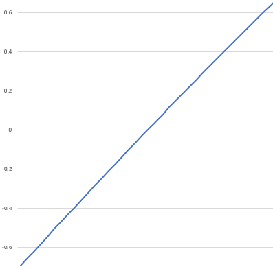
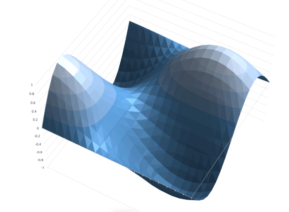
We understand that the derivative of an analytic function f(x) that takes a real and produces a real is the function f'(x) that gives the slope of f(x) at each point. But suppose we have a function that takes two reals and produces a real. Maybe f(x, y) = cos(x/5) sin(y/3). Here, I’ll graph that function from (0, 0) to (20, 20):

We could implement this in C# easily enough:

static ℝ Compute2(ℝ x, ℝ y) => Math.Cos(x / 5.0) * Math.Sin(y / 3.0);

That’s a pretty straightforward analytic function of two variables, but we’re programmers; we can think of two-variable functions as a one-variable factory that produces one-variable functions. (This technique is called currying, after the logician Haskell Curry.)

static Func<ℝ, ℝ> Compute2FromX(ℝ x) => (ℝ y) =>
  Math.Cos(x / 5.0) * Math.Sin(y / 3.0);

That is, given a value for x, we get back a function f(y), and now we are back in the world of single-variable real-to-real functions. We could then take the derivative of this thing with respect to y and find the slope “in the y direction” at a given (x, y) point.

Similarly we could go in the other direction:

static Func<ℝ, ℝ> Compute2FromY(ℝ y) => (ℝ x) =>
  Math.Cos(x / 5.0) * Math.Sin(y / 3.0);

And now given a “fixed” y coordinate we can find the corresponding function in x, and compute the slope “in the x direction”.

In wacky calculus notation, we’d say that ∂f(x, y)/∂x is the two-variable function that restricts f(x, y) to a specific y and computes the slope of that one-variable function in the x direction. Similarly ∂f(x, y)/∂y is the function that restricts f(x, y) to a specific x and computes the slope of that one-variable function in the y direction.

You probably see how we could compute the partial derivatives of a two-variable, real-valued analytic function using our Dual type; just curry the two-variable function into two one-variable functions, change all of the “doubles” to “Duals” in the “returned” function, and provide dualized implementations of sine and cosine.

But… do we actually need to do the currying step? It turns out no! We do need implementations of sine and cosine; as we discussed last time, they are:

public static ⅅ Cos(ⅅ x) =>
  new ⅅ(Math.Cos(x.r), –Math.Sin(x.r) * x.ε);
public static ⅅ Sin(ⅅ x) =>
  new ⅅ(Math.Sin(x.r), Math.Cos(x.r) * x.ε);

Easy peasy. We can now write our computation in non-curried, dualized form:

static ⅅ Compute2(ⅅ x, ⅅ y) => ⅅ.Cos(x / 5.0) * ⅅ.Sin(y / 3.0);

Now suppose we are interested in the x-direction slope and the y-direction slope at (13, 12), which is part of the way up the slope of the right hand “hill” in the graph:

Console.WriteLine(Compute2(13 + ⅅ.EpsilonOne, 12));
Console.WriteLine(Compute2(13, 12 + ⅅ.EpsilonOne));

We do the computation twice, and tell the compute engine to vary one-epsilon in the x direction the first time, and not at all in the y direction. The second time, we vary by one-epsilon in the y direction but not at all in the x direction. The output is:


0.648495546750919+0.0780265449058288ε
0.648495546750919+0.186699955809795ε


Which gives us that the slope in the x direction is about 0.078, and the slope in the y direction is about 0.187. So for the cost of computing the function twice, we can get the derivatives in both directions. Moreover, if we wanted to compute the slope in some other direction than “parallel to the x axis” or “parallel to the y axis”, perhaps you can see how we’d do that.

But we’ve actually gotten something even a bit more interesting and useful here: we’ve computed the gradient!

The gradient of a multivariate function like this one is the direction you’d have to walk to gain altitude the fastest. That is, if you are standing at point (13, 12) on that graph, and you walk 0.078 steps in the x direction for every 0.187 steps in the y direction, you’ll be heading in the “steepest” direction, which is the direction likely to get you to the top of the mountain the fastest:

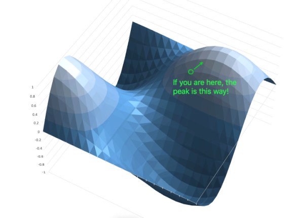
And of course if you walk in the “negative of the gradient” direction, you’re heading “downslope” as fast as possible.

Notice that heading in the “upslope” or “downslope” direction does not necessarily move you directly towards the nearest peak, valley or saddle; it heads you in the direction that is gaining or losing altitude the fastest. If you do not know exactly where the peaks and valleys are, that’s your best guess of the right direction to go.

I hope it is clear that there is no reason why this should be limited to functions of two variables, even though it is hard to visualize higher-dimensional functions! We can have a real-valued function of any number of variables, take the partial derivatives of each, and find the gradient that points us in the “steepest” direction.

Why is this useful? Well, imagine you have some very complicated but smooth multivariate function that represents, say, the cost of a particular operation which you would like to minimize. We might make an informed guess via some heuristic that a particular point is near a “cost valley”, and then compute the gradient at that point; this gives us a hint as to the direction of the nearest valley, and we can then try another, even more informed guess until we find a place where all the gradients are very small.  Or, equivalently, we might have a “benefit function” that we are trying to maximize, and we need a hint as to what direction the nearby peaks are. These techniques are in general called “gradient descent” and “gradient ascent” methods and they are quite useful in practice for finding local minima and maxima.

The point is: as long as the function you are computing is computed only by adding, subtracting, multiplying, and dividing doubles, or using double-valued library functions whose derivatives you know, you can “lift” the function to duals with only a minor code change, and then you get the derivative of that function computed exactly, for a very small additional cost per computation. That covers a lot of functions where it might not be at all obvious how to compute the derivative. Even better, for an n-dimensional function we can compute the gradient for only a cost of O(n) additional operations. (And in fact there are even more efficient ways to use dual numbers do this computation, but I’m not going to discuss them in this series.)

A great example of a high-dimensional computation that only uses real addition and multiplication is the evaluation of a function represented by a neural net in a machine learning application; by automatically differentiating a neural network during the training step, we can very efficiently tweak the neuron weights during the training step to seek a local maximum in the fitness of the network to the given task. But I think I will leave that discussion for another day.

Next time on FAIC: What exactly does A()[B()]=C(); do in C#? It might seem straightforward, but there are some subtle corner cases.

Last time on FAIC we discovered that when you “lift” a polynomial on doubles to a polynomial on duals and then evaluate it with x+1ε, the “real” part of the returned dual exactly corresponds to the original polynomial at x; that’s not a surprise. What is bizarre and fascinating is that the “epsilon” part of the dual exactly corresponds to the derivative of the polynomial at x!

First question: is this actually true for all polynomials, or did I trick you by choosing an example that just happened to work? Let’s make a little chart. I’ll make a bunch of power functions, and we’ll list the function, its derivative, and what happens if we lift the function to dual numbers and evaluate it on an arbitrary dual number:

    f(x)      f'(x)      f(a+bε)
     1          0          1+0ε
     x          1          a+bε
     x2         2x         a2+2abε  (The higher power ε terms vanish)
     x3         3x2        a3+3a2bε
     ...
     xn         nxn-1      an+nan-1bε
     ...

It sure looks like for every power function, f(a+bε) = f(a) + f'(a)bε. (Exercise: prove this by induction on the power.) And moreover, we could pretty easily show that this is true for all finite sums of these things, and all scalar multiplications, and therefore true for all polynomials.

Is it true for other functions? We know that f(x) = ex is defined as the limit of the infinite sum

1 + x + x2/2! + x3/3! ... 

and that moreover, f(x) = f'(x). So what then is f(a+bε) ?

ea+bε = 1 + a+bε + (a2+2abε)/2! + (a3+3a2bε)/3! ... 
= (1 + a + a2/2! + ...) + (1 + a + a2/2! + ...)bε
= ea + eabε
= f(a) + f'(a)bε

It’s nice that this falls right out of the definition; we could also have gotten there faster by using this property of exponentiation:

ea+bε = eaebε
= ea(1 + bε)   because the higher terms are all zero!
= f(a) + f'(a)bε

I will not labour the point; using similar tricks we can show:

ln(a+bε) = ln(a) + (1/a)bε
cos(a+bε) = cos(a) - sin(a)bε
sin(a+bε) = sin(a) + cos(a)bε

And since yx = ex ln y, we can now compute arbitrary powers of dual numbers as well.

In every case we find that for a function f(x) defined on reals, the “lifted” function on duals is f(a+bε) = f(a) + f'(a)bε. Now, to be strictly accurate, we need to put some limitations on the function. For example, its derivative has to exist! In fact we will be more restrictive than that, and limit the functions we consider to the “analytic” functions, which have the properties necessary to be amenable to calculus: they must be smooth, their first, second, third, … derivatives must exist, and so on. We don’t want to consider fractal curves or functions that come to sharp points, or have infinite slope at a point, or whatever. Just normal, everyday curves.

That all said, it still seems a little bit like magic that by lifting an ordinary function on doubles to a function on duals, we get a computation of both the function and its derivative at a point for almost free; there’s only an O(1) additional cost in time and memory to compute the derivative. This stands in contrast to the more traditional way of numerically approximating a derivative by repeatedly evaluating nearby points until the slope converges, which can involve many repeated computations and results in an approximation. Is there some intuitive explanation of why this works?

The intuition that works for me is: every analytic function is approximately a straight line if you restrict its range. Here’s our polynomial again, but this time graphed from -0.8 to -0.7. It’s nigh indistinguishable from a straight line over this range. But what straight line?

Well, the straight line that goes through (-0.75, f(-0.75)) and has slope of f'(-0.75) obviously! Thus it should not be a surprise that f(-0.75 + bε) should be f(-0.75) + f'(-0.75)bε. We’re essentially waving our hands here and saying that ε is so small that we can approximate the function in the neighbourhood of -0.75 as a straight line.

Next time on FAIC: Can we do some slightly more complicated calculus with this technique?

Last time on FAIC I introduced a fun variation on complex numbers called “dual numbers” consisting of a value “plus a tiny bit” notated as ε, where the really tiny part has the interesting property that ε2 is zero.

Well, enough chit-chat; let’s implement them.

You know what, just for grins I’m going to make this look a bit more like math, and a bit more concise while we’re at it:

using ⅅ = Dual;
using ℝ = System.Double;

(Unfortunately 𝔻 is not a legal identifier in C#.)

A dual is logically a value that consists of two doubles, so it makes sense to represent them as an immutable value type:

public struct Dual : IComparable<Dual>
{
  public ℝ Real { get; }
  public ℝ Epsilon { get; }
  public ℝ r => this.Real;
  public ℝ ε => this.Epsilon;

I got so sick of typing out “Real” and “Epsilon” that I had to make these helper properties, even though they do not meet C# naming guidelines. Guidelines are guidelines, not rules!

Notice also that, fun fact, C# lets you use any non-surrogate-pair Unicode character classified as a letter in an identifier.

The constructor is as you’d expect, and I’m going to make a helper property for 0+1ε:

public Dual(ℝ real, ℝ epsilon)
{
  this.Real = real;
  this.Epsilon = epsilon;
}
public static ⅅ EpsilonOne = new ⅅ(0, 1);

The math is as we’ve discussed:

public static ⅅ operator +(ⅅ x) => x;
public static ⅅ operator –(ⅅ x) => new ⅅ(–x.r, –x.ε);
public static ⅅ operator +(ⅅ x, ⅅ y) =>
  new ⅅ(x.r + y.r, x.ε + y.ε);
public static ⅅ operator –(ⅅ x, ⅅ y) =>
  new ⅅ(x.r – y.r, x.ε – y.ε);
public static ⅅ operator *(ⅅ x, ⅅ y) =>
  new ⅅ(x.r * y.r, x.ε * y.r + x.r * y.ε);
public static ⅅ operator /(ⅅ x, ⅅ y) =>
  new ⅅ(x.r / y.r, (x.ε * y.r – x.r * y.ε) / (y.r * y.r));

So easy!

UPDATE: I was WRONG WRONG WRONG in the section which follows.

An earlier version of this episode suggested that we implement comparisons on dual numbers as “compare the real parts; if equal, compare the epsilon parts”. But upon reflection, I think that’s not right. One of the characteristics of dual numbers that we like is that “lifting” a computation on reals to dual numbers produce the same “real part” in the result. Suppose we have:

static bool Foo(ℝ x) => x > 2.0;

Then we reasonably expect that

static bool  Foo(ⅅ x) => x > 2.0;

agrees with it, no matter what value we have for epsilon.

So I’m going to tweak the code so that we compare only real parts.

Resuming now the original episode…

My preference is to implement the logic in one place in a helper, and then call that helper everywhere:

private static int CompareTo(ⅅ x, ⅅ y) =>
  x.r.CompareTo(y.r);
public int CompareTo(ⅅ x) =>
  CompareTo(this, x);
public static bool operator <(ⅅ x, ⅅ y) =>
  CompareTo(x, y) < 0;
public static bool operator >(ⅅ x, ⅅ y) =>
  CompareTo(x, y) > 0;
public static bool operator <=(ⅅ x, ⅅ y) =>
  CompareTo(x, y) <= 0;
public static bool operator >=(ⅅ x, ⅅ y) =>
  CompareTo(x, y) >= 0;
public static bool operator ==(ⅅ x, ⅅ y) =>
  CompareTo(x, y) == 0;
public static bool operator !=(ⅅ x, ⅅ y) =>
  CompareTo(x, y) != 0;
public bool Equals(ⅅ x) =>
CompareTo(this, x) == 0;
public override bool Equals(object obj) =>
  obj is ⅅ x && CompareTo(this, x) == 0;

And finally, a few loose ends. It would be nice to be able to convert to Dual from double automatically, and we should also override ToString and GetHashCode just to be good citizens:

public static implicit operator ⅅ(ℝ x) => new ⅅ(x, 0);
public override string ToString() => $”{r}{(ε<0.0?“”:“+”)}{ε}ε”;
public override int GetHashCode() => r.GetHashCode();

Super, that was really easy. And now we can take any old method that does math on doubles, and make it do math on Duals. Suppose we’ve got this little guy, that computes x4+2x3-12x2-2x+6:

static ℝ Compute(ℝ x) =>
  x * x * x * x + 2 * x * x * x – 12 * x * x – 2 * x + 6;

If we just turn all the doubles into Duals:

static ⅅ Compute(ⅅ x) =>
  x * x * x * x + 2 * x * x * x – 12 * x * x – 2 * x + 6;

Then we have the same function, but now implemented in the dual number system. This:

Console.WriteLine(Compute(1.0 + Dual.EpsilonOne));

Produces the output -5-16ε, which agrees with the original method in the real part, and is -16 in the epsilon part. Apparently computing that polynomial with one plus a tiny amount gives us -5, plus -16 “more tiny amounts”.

Hmm.

You know what, just for grins I’m going to compute this function from -4.5+εto 3.5+ε and then graph the real and epsilon parts of the output of our “dualized” function.

The blue line is the real part, the orange line is the epsilon part. As we expect, the blue line corresponds to the original polynomial. But the orange line looks suspiciously familiar…

HOLY GOODNESS THE ORANGE LINE IS ZERO WHERE THE BLUE LINE IS FLAT.

The epsilon part is the derivative of the polynomial!

Next time on FAIC: How’d that happen?

I’ve recently been looking into a fascinating corner of mathematics that at first glance appears a little bit silly, but actually has far-reaching applications, from physics to numerical methods to machine learning. I thought I’d share what I’ve learned over the next few episodes.

I assume you recall what a complex number is, but perhaps not all of the details. A complex number is usually introduced as a pair of real numbers (a, b), where a is called the “real part” and b is called the “imaginary part”.

A brief aside: it has always bugged me that these labels are unnecessarily value-laden. There is no particular “reality” that is associated with the real part; it is every bit as “imaginary” as the imaginary part. They might as well be called the “rezrov part” and the “gnusto part”, but we’re stuck with “real” and “imaginary”. Moving on.

It would be perfectly sensible to notate these as a pair (a, b) — and indeed, when we characterize complex numbers as points on the complex plane, we often do. But it is also convenient to notate complex numbers in an algebraic form a+bi, where the i indicates the imaginary part.

Finally, we have well-known rules for adding and multiplying complex numbers. The fundamental rule is that (0+1i)2 is equal to -1+0i, and the rest of the rules follow from there. For complex numbers:

(a+bi) + (c+di) = (a+c) + (b+d)i
(a+bi)(c+di)    = (ac-bd) + (ad+bc)i

Division is a little bit tricky and I won’t write it all out here; look it up if you do not remember. We can similarly go on to derive rules for complex exponentiation, trigonometry, and so on.

Let’s switch gears slightly. It is very common in mathematics, and especially calculus, to reason about a quantity “plus a little bit”. That is, any old quantity, plus some positive amount that is not zero, but is much smaller than one, and really, really small compared to the original quantity. What “really, really small” means is of course dependent on context; maybe one-millionth of the original quantity is small. Maybe one-millionth is still pretty big, but one-trillionth, or one part in a googolplex, or whatever, is “really small” in our context. I’m being deliberately vague and hand-wavy here; just run with it.

Let’s call our really small positive quantity ε, which is the lower-case Greek letter epsilon; it is traditionally used in calculus to represent a very small quantity. Let’s suppose our value is a, and we have a very small amount added to it, so that would be a+ε. Hmm. What if we doubled that quantity? Plainly that would be 2a+2ε. So scalar multiplication works as you’d expect. It seems reasonable that if we can have 2ε then we can have 3ε or for that matter 3.14ε or bε for any real value of b. So once again we have an (a, b) pair of numbers representing a quantity, which we notate as a+bε. What are the algebraic rules of this thing? It certainly makes sense that addition should work as we expect, the same as complex addition:

(a+bε) + (c+dε) = (a+c) + (b+d)ε

This should match our intuitions. The sum of “a plus a bit” and “c plus a bit” should be “a + c plus a bit” if there is justice in the world. What about multiplication? Let’s just multiply it out using ordinary algebra:

(a+bε)(c+dε) = ac + (ad+bc)ε + bdε2

We seem to have introduced an ε2 term there. What are we going to do with that? Remember, ε is not zero but is very, very small indeed, so that thing squared must be super tiny. So tiny that we can just ignore it entirely! (Remember, I am hand-waving egregiously here.) Let’s just say that ε2 is by definition zero, just as we said that i2 is by definition -1, and see what happens. So we have:

(a+bε)(c+dε) = ac + (ad+bc)ε

Again, this should match our intuitions. The product of something a bit bigger than a with something a bit bigger than c should be a bit bigger than the product of a and c.

What about division? Division by zero is illegal, and division by zero plus a tiny amount I think should also be illegal. Seems reasonable. What then is (a+bε)/(c+dε) when c is not zero? Well, if it is not zero then we can multiply top and bottom by c-dε:

a+bε   (c-dε)(a+bε)   ac + (bc-da)ε    a   bc-da
———— = ——————————— = —————————————— = - + ————— ε
c+dε   (c-dε)(c+dε)       c2           c     c2

Once again our intuition is satisfied: the quotient of “something close to a” divided by “something close to c” is close to the quotient of a and c.

This is a pretty neat number system; it is called the dual number system and it was introduced to the world in 1873 by the English mathematician William Clifford. But so far it might look like it is just a curiosity; however, it is extremely useful.

Next time on FAIC: we will implement the dual number system in C#, and discover a surprising property.

Happy New Year all and welcome to another year of having fabulous adventures in coding. I thought I’d start this year off by answering a question I get quite frequently:

I have a public outer class with a public nested class. The nested class represents a concept only meaningful in the context of the outer class, and it accesses private members of the outer class. I want some of the members of the nested class to be public to everyone, but I want some of them to be public only to the outer class; how can I do that?

Typically the members they want to be accessible only to the containing class to be things like property setters and constructors:

public class Outer
{
  public class Inner
  {
    // I want the ctor and setter to be accessible in Outer
    // but not to the general public.
    public Inner() { ... }
    public Foo Foo { get; set; } 
    // whatever ... 
  }
  public Inner Frob() { ... }
  // ... and so on ...
}

I can think of four ways to solve this problem offhand, though I’m sure there are more.

Attempt one: my preferred solution is to deny the premise of the question and make the “private” details that need to be used by the container “internal”. It is your assembly! If you don’t want to abuse the internal details outside of a particular class, then don’t do it. If your coworkers do it, educate them in code reviews. Not every authorial intention needs to be expressed in the accessibility system, after all.

Attempt two: again, deny the premise of the question, but this time make the nested type a private implementation detail. The received wisdom is that we want nested classes to be private implementation details of the public outer class, not themselves public classes. In that case you’d simply make an interface to expose the public details:

public interface IFoo
{
  public Foo Foo { get; }
}
public class Outer
{
  private class Inner : IFoo
  {
    public Inner() { ... }
    public Foo Foo { get; private set; } 
    // whatever ... 
  }
  public IFoo Frob() { ... }
  // ... and so on ...
}

This has a couple of down sides though. We’ve denied the premise of the question, which is that the nested class makes sense to be public, and so not answered the question. We’ve also “polluted” the public namespace by adding a new IFoo concept unnecessarily. Also, there is now the possibility that just anyone can create an implementation of IFoo. Typically in these sorts of scenarios, the reason we want to restrict the constructor and setter is to ensure that the invariants of the inner type are being guaranteed by the code in the outer type.

Attempt three: did you know that it is legal for a type to implement an interface that is less public than the type? That is not true for base types, but it is true for interfaces!

public class Outer
{
  private interface IFooSetter
  {
    public Foo Foo { set; }
  }
  public class Inner : IFooSetter
  {
    public Inner() { ... }
    public Foo Foo { get; private set; } 
    Foo IFooSetter.Foo { set { this.Foo = value; } }
    // whatever ... 
  }
  public Inner Frob() { ... }
  // ... and so on ...
}

Now code in Outer can cast an Inner to IFooSetter and call the setter that way, but code outside of Outer cannot cast to IFooSetter because that type is private to Outer.

This looks pretty good, but again we’ve got a few problems. We still haven’t dealt with the constructor problem. And in both the solutions we’ve seen so far, it works poorly in the case where the inner type is a value type because we end up boxing.  Yes, it is a very bad practice to make a mutable value type, but hey, that’s probably why we’re restricting the mutators to be only accessible from Outer! Regardless though, we’d like a way to avoid the boxing penalty.

Attempt four: avoid interfaces altogether and go straight to delegates:

// This code is wrong!
public class Outer
{
  private static Func<Inner> innerFactory = null;
  private static Action<Inner, Foo> fooSetter = null;
  public class Inner
  {
    static Inner() 
    {
      Outer.innerFactory = ()=>new Inner();
      Outer.fooSetter = (i, f)=>i.Foo = f;
    }
    private Inner() { ... }
    public Foo Foo { get; private set; } 
    // ...
  }
  public Inner Frob() => innerFactory();
  // ... and so on ...
}

Now code in Outer can call innerFactory() any time it needs an Inner, and can call fooSetter(inner, foo) any time it needs to call a setter on an Inner.

I’ll leave you with two exercises:

• First, the code above is wrong because it can be easily made to crash; do you see how? Can you fix it? (Hint: there is no way using just the rules of C# that I know of; you need to use a special method created for compiler writers.)
• Second, suppose the inner type is a mutable value type; our setter would mutate a copy. Can you fix that too?