You might recall that before my immensely long series on ways we could make C# a probabilistic programming language, I did a short series on how we can automatically computed the exact derivative in any direction of a real-valued function of any number of variables for a small cost, by using dual numbers. All we need is for the function we are computing to be computed by addition, subtraction, multiplication, division and exponentiation of functions whose derivatives are known, which is quite a lot of possible functions.

There is a reason why I did that topic before “Fixing Random”, but sadly I never got to the connection between differential calculus and sampling from an arbitrary distribution. I thought I might spend a couple of episodes sketching out how it is useful to use automatic differentiation when trying to sample from a distribution. I’m not going to write the code; I’ll just give some of the “flavour” of the algorithms.

Before I get into it, a quick refresher on the Metropolis algorithm. The algorithm is:

• We have a probability distribution function that takes a point and returns a double that is the “probability weight” of that point. The PDF need not be “normalized”; that is, the area under the curve need not add up to 1.0. We wish to generate a series of samples that conforms to this distribution.
• We choose a random “initial point” as the current sample.
• We randomly choose a candidate sample from some distribution based solely on the current sample.
• If the candidate is higher weight than current, it becomes the new current and we yield the value as the sample.
• If it is lower weight, then we take the ratio of candidate weight to current weight, which will be between 0.0 and 1.0. We flip an unfair coin with that probability of getting heads. Heads, we accept the candidate, tails we reject it and try again.
• Repeat; choose a new candidate based on the new current.

The Metropolis algorithm is straightforward and works, but it has a few problems.

• How do we choose the initial point?

Since Metropolis is typically used to compute a posterior distribution after an observation, and we typically have the prior distribution in hand, we can use the prior distribution as our source of the initial point.

• What if the initial point is accidentally in a low-probability region? We might produce a series of unlikely samples before we eventually get to a high-probability current point.

We can solve this by “burning” — discarding — some number of initial samples; we waste computation cycles so we would like the number of samples it takes to get to
“convergence” to the true distribution to be small. As we’ll see, there are ways we can use automatic differentiation to help solve this problem.

• What distribution should we use to choose the next candidate given the current sample?

This is a tricky problem. The examples I gave in this series were basically “choose a new point by sampling from a normal distribution where the mean is the current point”, which seems reasonable, but then you realize that the question has been begged. A normal distribution has two parameters: the mean and the standard deviation. The standard deviation corresponds to “how big a step should we typically try?”  If the deviation is too large then we will step from high-probability regions to low-probability regions frequently, which means that we discard a lot of candidates, which wastes time. If it is too small then we get “stuck” in a high-probability region and produce a lot of samples close to each other, which is also bad.

Basically, we have a “tuning parameter” in the standard deviation and it is not obvious how to choose it to get the right combination of good performance and uncorrelated samples.

These last two problems lead us to ask an important question: is there information we can obtain from the weight function that helps us choose a consistently better candidate? That would lower the time to convergence and might also result in fewer rejections when we’ve gotten to a high-probability region.

I’m going to sketch out one such technique in this episode, and another in the next.

As I noted above, Metropolis is frequently used to sample points from a high-dimensional distribution; to make it easier to understand, I’ll stick to one-dimensional cases here, but imagine that instead of a simple curve for our PDF, we have a complex multidimensional surface.

Let’s use as our motivating example the mixture model from many episodes ago:

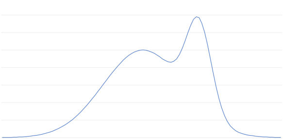
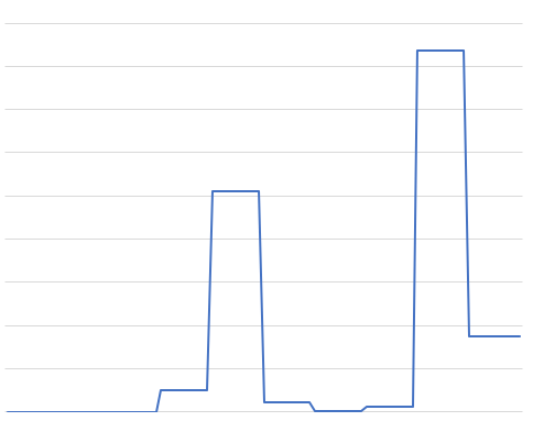
Of course we can sample from this distribution directly if we know that it is the sum of two normal distributions, but let’s suppose that we don’t know that. We just have a function which produces this weight.  Let me annotate this function to say where we want to go next if the current sample is in a particular region.

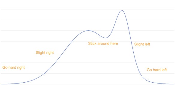
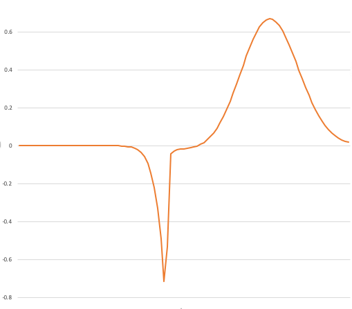
I said that we could use the derivative to help us, but it is very unclear from this diagram how the derivative helps:

• The derivative is small and positive in the region marked “go hard right” and in the immediate vicinity of the two peaks and one valley.
• The derivative is large and positive in the “slight right” region and to the left of the tall peak.
• The derivative is large and negative in the “slight left” region and on the right of the small peak.
• The derivative is small and negative in the “hard left” region and in the immediate vicinity of the peaks and valley.

No particular value for the derivative clearly identifies a region of interest. It seems like we cannot use the derivative to help us out here; what we really want is to move away from small-area regions and towards large-area regions.

Here’s the trick.

Ready?

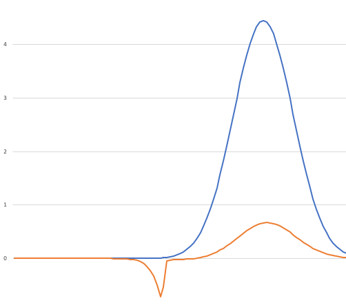
I’m going to graph the log of the weight function below the weight function:

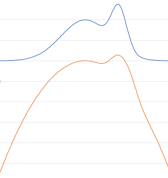
Now look at the slope of the log-weight. It is very positive in the “move hard right” region, and becomes more and more positive the farther left we go! Similarly in the “move hard left” region; the slope of the log-weight is very negative, and becomes more negative to the right.

In the “slight right” and “slight left” regions, the slope becomes more moderate, and when we are in the “stay around here” region, the slope of the log-weight is close to zero. This is what we want.

(ASIDE: Moreover, this is even more what we want because in realistic applications we often already have the log-weight function in hand, not the weight function. Log weights are convenient because you can represent arbitrarily small probabilities with “normal sized” numbers.)

We can then use this to modify our candidate proposal distribution as follows: rather than using a normal distribution centered on the current point to propose a candidate, we compute the derivative of the log of the weight function using dual numbers, and we use the size and sign of the slope to tweak the center of the proposal distribution.

That is, if our current point is far to the left, we see that the slope of the log-weight is very positive, so we move our proposal distribution some amount to the right, and then we are more likely to get a candidate value that is in a higher-probability region. But if our current point is in the middle, the slope of the log-weight is close to zero so we make only a small adjustment to the proposal distribution.

(And again, I want to emphasize: realistically we would be doing this in a high-dimensional space, not a one-dimensional space. We would compute the gradient — the direction in which the slope increases the most — and head that direction.)

If you work out the math, which I will not do here, the difference is as follows. Suppose our non-normalized weight function is p.

• In the plain-vanilla proposal algorithm we would use as our candidate distribution a normal centered on current with standard deviation s.
• In our modified version we would use as our candidate distribution a normal centered on current + (s / 2) * ∇log(p(current)), and standard deviation s.

Even without the math to justify it, this should seem reasonable. The typical step in the vanilla algorithm is on the order of the standard deviation; we’re making an adjustment towards the higher-probability region of about half a step if the slope is moderate, and a small number of steps if the slope is severe; the areas where the slope is severe are the most unlikely areas so we need to get out of them quickly.

If we do this, we end up doing more math on each step (to compute the log if we do not have it already, and the gradient) but we converge to the high-probability region much faster.

If you’ve been following along closely you might have noticed two issues that I seem to be ignoring.

First, we have not eliminated the need for the user to choose the tuning parameter s. Indeed, this only addresses one of the problems I identified earlier.

Second, the Metropolis algorithm requires for its correctness that the proposal distribution not ever be biased in one particular direction! But the whole point of this improvement is to bias the proposal towards the high-probability regions. Have I pulled a fast one here?

I have, but we can fix it. I mentioned in the original series that I would be discussing the Metropolis algorithm, which is the oldest and simplest version of this algorithm. In practice we use a variation on it called Metropolis-Hastings which adds a correction factor to allow non-symmetric proposal distributions.

The mechanism I’ve sketched out today is called the Metropolis Adjusted Langevin Algorithm and it is quite interesting. It turns out that this technique of “walk in the direction of the gradient plus a random offset” is also how physicists model movements of particles in a viscous fluid where the particle is being jostled by random molecule-scale motions in the fluid. (That is, by Brownian motion.) It’s nice to see that there is a physical interpretation in what would otherwise be a very abstract algorithm to produce samples.

Next time on FAIC: The fact that we have a connection to a real-world physical process here is somewhat inspiring. In the next episode I’ll give a sketch of another technique that uses ideas from physics to improve the accuracy of a Metropolis process.

Source code for this episode is here.

Welcome to this special bonus episode of Fixing Random, the immensely long blog series where I discuss ways to add probabilistic programming features into C#. I ran into an interesting problem at work that pertains to the techniques that we discussed in this series, so I thought I might discuss it a bit today.

Let’s suppose we have three forts, Fort Alpha, Fort Bravo and Fort Charlie at the base of a mountain. They are constantly passing messages back and forth by carrier pigeon. Alpha and Charlie are too far apart to fly a pigeon directly, so messages from Alpha to Charlie first go from Alpha to Bravo, and then on from Bravo to Charlie. (Similarly. messages from Charlie to Alpha go via Bravo, but we’ll not worry about that direction for the purposes of this discussion.)

Carrier pigeons are of course an unreliable mechanism for passing messages, so let’s model this as a Bernoulli process; every time we send a message from Alpha to Bravo, or Bravo to Charlie, we flip an unfair coin. Heads, the bird gets through, tails it gets lost along the way.

From this we can predict the reliability of passing a message from Alpha to Charlie via Bravo; the probability of failure is the probability that A-B fails or B-C fails (or both). Equivalently, the probability of success is the probability of A-B succeeding and B-C succeeding. This is just straightforward, basic probability; if the probability of success from A-B is, say, 95% and B-C is 96%, then the probability of success from A to C is their product, around 91%.

Aside: Note that I am assuming in this article that pigeons are passing from Bravo to Charlie even if a pigeon failed to arrive from Alpha; I’m not trying to model in this system constraints like “pigeons only fly from Bravo to Charlie when one arrived from Alpha”.

Now let’s add an extra bit of business.

We have an observer on the mountaintop at Fort Delta overlooking Alpha, Bravo and Charlie. Delta has some high-power binoculars and is recording carrier pigeon traffic from Alpha to Bravo and Bravo to Charlie. But here’s the thing: Delta is an unreliable observer, because observing carrier pigeons from a mountaintop is inherently error-prone; sometimes Delta will fail to see a pigeon. Let’s say that 98% of the time, Delta observes a pigeon that is there, and Delta never observes a pigeon that is not there.

Every so often, Delta issues a report: either “the channel from Alpha to Charlie is healthy” if Delta has observed a pigeon making it from Alpha to Bravo and also a pigeon making it from Bravo to Charlie. But if Delta has just failed to observe either a pigeon going from Alpha to Bravo, or a pigeon going from Bravo to Charlie, then Delta issues a report saying “the channel from Alpha to Charlie is unhealthy“.

The question now is: suppose Delta issues a report that the Alpha-Charlie channel is unhealthy. What is the probability that a pigeon failed to get from Alpha to Bravo, and what is the probability that a pigeon failed to get from Bravo to Charlie? Each is surely much higher than the 5-ish percent chance that is our prior.

We can use the gear we developed in the early part of my Fixing Random series to answer this question definitively, but before we do, make a prediction. If you recall episode 16, you’ll remember that you can have a 99% accurate test but the posterior probability of having the disease that the test diagnoses is only 50% when you test positive; this is a variation on that scenario.

Rather than defining multiple enumerated types as I did in earlier episodes, or even using bools, let’s just come up with a straightforward numeric encoding. We’ll say that 1 represents “a pigeon failed to make the journey”, and 0 means “a pigeon successfully made the journey” — if that seems backwards to you, I agree but it will make sense in a minute.

Similarly, we’ll say that 1 represents “Delta’s attempt to observe a pigeon has failed”, and 0 as success, and finally, that 1 represents Delta making the report “the channel is unhealthy” and 0 represents “the channel is healthy”.

The reason I’m using 1 in all these cases to mean “something failed” is because I want to use OR to get the final result. Let’s build our model:

var ab = Bernoulli.Distribution(95, 5);
var bc = Bernoulli.Distribution(96, 4);
var d = Bernoulli.Distribution(98, 2);

• 5% of the time ab reports 1: the pigeon failed to get through.
• 4% of the time, bcreports 1: the pigeon failed to get through.
• 2% of the time, d reports 1: it fails to see a pigeon that is there.

Now we can ask and answer our question about the posterior: what do we know about the posterior distribution of pigeons making it from Alpha to Bravo and Bravo to Charlie? We’ll sample from ab and bc once to find out if a pigeon failed to get through, and then ask whether Delta failed to observe the pigeons.

What is the condition that causes Delta to report that the channel is unhealthy?

• the pigeon from Alpha to Bravo failed, OR
• the pigeon from Bravo to Charlie failed, OR
• Delta failed to observe Alpha’s pigeon, OR
• Delta failed to observe Bravo’s pigeon.

We observe that Delta reports that the channel is unhealthy, so we’ll add a where clause to condition the result, and then print out the resulting posterior joint probability:

var result = from pab in ab
             from pbc in bc
             from oab in d
             from obc in d
             let report = pab | pbc | oab | obc
             where report == 1
             select (pab, pbc);
Console.WriteLine(result.ShowWeights());

This is one of several possible variations on the “noisy OR distribution” — that is, the distribution that we get when we OR together a bunch of random Boolean quantities, but where the OR operation itself has some probabilistic “noise” attached to it.

Aside: That’s why I wanted to express this in terms of OR-ing together quantities; of course we can always turn this into a “noisy AND” by doing the appropriate arithmetic, but typically this distribution is called “noisy OR”.

We get these results:

(0, 0):11286    -- about 29%
(0, 1):11875    -- about 30%
(1, 0):15000    -- about 39%
(1, 1):625      -- less than 2%

Remember that (0, 0) means that pigeons did make it from Alpha to Bravo and from Bravo to Charlie; in every other case we had at least one failure.

It should not be too surprising that (1, 1) — both the Alpha and Bravo pigeons failed simultaneously — is the rarest case because after all, that happens less than 9% of the cases overall, so it certainly should happen in some smaller percentage of the “unhealthy report” cases.

But the possibly surprising result is: when Delta reports a failure, there is a 29% chance that this is a false positive report of failure, and in fact it is almost as likely to be a false positive as it is to be a dropped packet, I mean lost pigeon, between Bravo and Charlie!

Put another way, if you get an “unhealthy” report, 3 times out of 10, the report is wrong and you’ll be chasing a wild goose. Just as we saw with false positives for tests for diseases, if the test failure rate is close to the disease rate of the population, then false positives make up a huge percentage of all positives.

My slip-up there of course illuminates what you figured out long ago; all of this whimsy about forts and pigeons and mountains is just a silly analogy. Of course what we really have is not three forts connected by two carrier pigeon routes, but ten thousand machines and hundreds of routers in a data center connected by network cabling in a known topology. Instead of pigeons we have trillions of packets. Instead of an observer in a fort on a mountaintop, we have special supervising software or hardware that is trying to detect failures in the network so that they can be diagnosed and fixed. Since the failure detection system is itself part of the network, it also is unreliable, which introduces “noise” into the system.

The real question at hand is: given prior probabilities on the reliability of each part of the system including the reporting system itself, what are the most likely posterior probabilities that explain a report that some part of the network is unhealthy?

This is a highly practical and interesting question to answer because it means that network engineers can quickly narrow down the list of possible faulty components given a failure report to the most likely culprits.  The power of probabilistic extensions in programming languages is that we now have the tools that we need to concisely express both those models and the observations that we need explanations for, and then generate the answers automatically.

Of course I have just given some of the flavor of this problem space and I’m sure you can imagine a dozen ways to make the problem more interesting:

• what if instead of a coin flip that represent “dropped” or “delivered” on a packet, we had a more complex distribution on every edge of the network topology graph — say, representing average throughput?
• How does moving to a system with continuous probabilities change our analysis and the cost of producing that analysis?
• And so on.

We can use the more complex tools I developed in my series, like the Metropolis method, to solve these harder problems; however, I think I’ll leave it at that for now.

All right, let’s finish this thing off!

First, I want to summarize, second I want to describe a whole lot of interesting stuff that I did not get to, and third, I want to give a selection of papers and further reading that inspired me in this series.

If you come away with nothing else from this series, the key message is: probabilistic programming is important, it is too hard today, and we can do a lot better than we are doing. We need to build better tools that leverage the type system and support line-of-business programmers who need to do probabilistic work, the same way that we built better tools for programmers who needed to use sequences, or databases, or asynchrony.

• We started this series with me complaining about System.Random, hence the name of the series. Even though some of the implementation details have finally improved after only some decades of misleading developers, we are still dealing with random numbers like it was 1972.
• The abstraction that we’re missing is to make “value drawn from a random distribution” a part of the type system, the same way that “function that returns a value”, or “sequence of values”, or “value that might be null” is part of the type system.
• The type we want is something like a sequence enumeration, but instead of a “move next” operation, we’ve got a “sample” operation.
• If we stick to simple distributions where the support is finite and small and the “weights” are integers, and restrict ourselves to pure functions, we can create new distributions from old ones using the same operations that we use to create new sequences from old ones: the LINQ operators Select, SelectMany and Where.
• Moreover, we can compute distributions exactly at runtime, without doing rejection sampling or other clever techniques.
• And we can even use query comprehension syntax, which makes me happy.
• From this we can see that probability distributions are monads; P(A) is just IDistribution<A>
• We also see that conditional probabilities P(B given A) are just Func<A, IDistribution<B>> — they are likelihood functions.
• The SelectManyoperation on the probability monad lets us combine a likelihood function with a prior probability.
• The Where operation lets us compute a posterior given a prior, a likelihood and an observation.
• This is an extremely useful result; even domain experts like doctors often do not have good intuitions about how an observation should change our opinions about the probability of an event having occurred. A positive result on a test of a rare disease may be only weak evidence if the test failure rate is close to the disease rate.
• Can we put these features in the language as well as the type system? Abusing LINQ is clever but maybe not the best from a usability perspective.
• We could in fact embed sample and condition operators in the C# language, just as we embedded await. We can then write an imperative workflow, and have the compiler generate a method that returns the correct probability distribution, just as await allows us to write an asynchronous workflow and the compiler generates a method that returns a task!
• Unfortunately, real-world probability problems are seldom discrete, small, and completely analyzable; they’re more often continuous and approximated.
• Implementing Sample efficiently on arbitrary distributions turns out to be a hard problem.
• We can use our tools to generate Markov chains.
• We can use Markov chains to implement Sample using the Metropolis Algorithm
• If we have a continuous prior (like a mint that produces coins of a certain quality with a certain probability) and a discrete likelihood (like the probability of a coin flip coming up heads), we can use this technique to compute a continuous posterior given an observation of one or more flips.
• This is a very useful technique in many real-world applications.
• Computing the expected value of a distribution given a function is a tricky problem in of itself, but there are a variety of techniques we can use.
• And if we can do that, we can solve some high-dimensional integral calculus problems!

That was rather a lot, and we still did not get to everything I wanted to.

By far the biggest thing that I did not get to, and that I may return to in another series of posts, is: the connection between await as an operator and sampleas an operator  is deeper than you might think.

As I noted above, you can put sample and condition operations in a language and have the compiler build a method that when run, generates a simple, discrete distribution. But it turns out we can actually do a pretty good job of dealing with sample operators on non-discrete distributions as well, by having the compiler be smart about using some of the techniques that we discussed in this series for continuous distributions.

What you really need is the ability to pick a sample, run a little bit of a routine, remember the result, back up a bit and try a different sample, and so on; from this we can build a distribution of program traces, and from that we can build an approximation of the distribution of the output of a probabilistic method!

This kind of control flow is tricky; it’s sort of a generalization of coroutines where you’re allowed to re-run code that you’ve run before, but with different values for the variables to see what happens.

Obviously it is crucially important that the methods be pure! It’s also crucially important that you spend most of your time exploring high-likelihood control flows, because the number of unlikely control flows is nigh infinite. If this sounds a bit like training up an ML model and then using that model in production later, that’s because it is basically the same thing, but applied to programs.

I know what you’re thinking: that sounds bonkers. But —  here is the thing that really got me motivated to write this series in the first place — we actually did it.

A while back my colleague Michael and I hacked together (ha ha) an implementation of multi-shot-continuations for Hack, our PHP variant and showed that we could in fact do probabilistic workflows where we have a distribution, and we sample from it some number of times, and trace out what happens in the program as we do so.

I then went on to work on other projects, but in the meanwhile a team of people who understand statistics far, far better than I do actually built an industrial-strength probabilistic control flow language with a sample operator. 

You can read all about it at their paper Hack PPL: A Universal Probabilistic Programming Language.

Another point that I very much wanted to get to in this series but did not is: we can do the same thing in C#, and in fact we can do it today.

The C# team added the ability to return types other than Task<T> from asynchronous workflows; and it turns out you only need to abuse that feature a small amount to convince C# to “go back a bit” in the workflow – back to the previous await operation, which becomes a stand-in for sample — and re-run portions of it with different sampled values. The C# team could add probabilistic workflows to C# tomorrow.

The C# team has historically done a great job of finding useful monads and embedding them into the control flow of the language; monadic probabilistic workflows with multi-shot continuations could be the next one. How about it team?

Finally, here’s a very incomplete list of papers and web sites that were inspiring to me in writing this series. I learned a lot, and there is plenty more to learn; I’ve just scratched the surface here.

• The idea that we can treat probability distributions like LINQ queries was given to me by my friend and director Erik Meijer; his fun and accessible paper Making Money Using Math hits many of the same points I did in this series, but I did it with a lot more code.
• The design of coroutines in Kotlin was a great inspiration to me; they’ve done a great job of making features that you would normally think of as being part of the language proper, like yield and await, into library methods. The first thing I did in my multi-shot coroutine hack was verify that I could simulate those features. (I was also very pleased to discover that much of this work was implemented by my old colleague Nikov from the C# team!)
• An introduction to probabilistic programming is a book-length work that uses a Lisp-like language with sample and observe primitives.
• Church is another Lisp-like language often used in academic studies of PPLs.
• The webppl.org web site has a Javascript-based implementation of a probabilistic programming language and a lot of great supporting information at dippl.org.

The next few papers are more technical.

• Build Your Own Probability Monads is a good overview for the Haskell programmers out there, as are Practical Probabilistic Programming With Monads and   Stochastic Lambda Calculus and Monads of Probability Distributions.
• Lightweight Implementations of Probabilistic Programming Languages Via Transformational Compilation is a good overview of how you can use MCMC techniques on program traces. A provably correct sampler for probabilistic programs goes into some of the correctness problems faced by PPL implementations, and Generating Efficient MCMC Kernels goes into some of the performance problems.
• Another fascinating area that I wanted to explore in this series is: we know it is bad enough to try to debug programs that have yields and awaits in them; how on earth do you debug programs that are actually running the same code paths maybe thousands of times when exploring the sample space of a workflow? Here’s an interesting paper on debugging probabilistic workflows.

And these are some good ones for the math:

• These MIT course notes on Bayesian updating of continuous priors was a good primer for my episodes on coin flipping. And the lecture notes MC Methods and Importance Sampling are what it says on the tin.
• Understanding the Metropolis-Hastings Algorithm gives a bunch of the underlying math.
• The enormous book Information Theory, Inference and Learning Algorithms was invaluable in getting me up to speed on math I had not done since my undergrad days.

There are many more that I am forgetting, and I’ll add to this list as I recall them.

All right, that was super fun; I am off on my annual vacation where I have no phone or internet, so I’m going to take a bit of a break from blogging; we’ll see you in a month or so for more fabulous adventures in coding!

Let’s sum up the last few episodes:

Suppose we have a distribution of doubles, p, and a function f from double to double. We often want to answer the question “what is the average value of f when it is given samples from p?” This quantity is called the expected value.

The obvious (or “naive”) way to do it is: take a bunch of samples, evaluate the function on those samples, take the average. Easy! However, this can lead to problems if there are “black swans”: values that are rarely sampled, but massively affect the value of the average when run through f. We would like to get a good estimate without having to massively increase the number of samples in our average.

We developed two techniques to estimate the expected value:

First, abandon sampling entirely and do numerical integral calculus:

• Use quadrature to compute two areas: the area under f(x)*p.Weight(x)  and the area under p.Weight(x) (which is the normalization constant of p)
• Their quotient is an extremely accurate estimate of the expected value
• But we have to know what region to do quadrature over.

Second, use importance sampling:

• Find a helper distribution q whose weight is large where f(x)*p.Weight(x) bounds a lot of area.
• Use the naive algorithm to estimate the expected value of  x=>f(x)*p.Weight(x)/q.Weight(x)from samples of q
• That is proportional to the expected value of f with respect to p
• We gave a technique for estimating the proportionality constant by sampling from q also.

The problem with importance sampling then is finding a good q. We discussed some techniques:

• If you know the range, just use a uniform distribution over that range.
• Stretch and shift p so that the transformed PDF doesn’t have a “black swan”, but the normalization constant is the same.
• Use the Metropolis algorithm to generate a helper PDF from Abs(f*p), though in my experiments this worked poorly
• If we know the range of interest, we can use the VEGAS algorithm. It makes cheap, naive estimates of the area of subranges, and then uses that information to gradually refine a piecewise-uniform helper PDF that targets spikes and avoid flat areas of f*p.
• However, the VEGAS algorithm is complex, and I did not attempt to implement it for this series.

The question you may have been asking yourself these past few episodes is:

If quadrature is an accurate and cheap way to estimate the expected value of f over samples from p then why are we even considering doing sampling at all? Surely we typically know at least approximately the range over which f*p has some area. What’s the point of all this?

Quadrature just splits up the range into some number — say, a thousand — equally-sized pieces, evaluates f*p on each of them, and takes the average. That sure seems cheaper and easier than all this mucking around with sampling. Have I just been wasting your time these past few episodes? And why has there been so much research and effort put into finding techniques for estimating expected value?

This series is called “Fixing Random” because the built-in base class library tools we have in C# for representing probabilities are weak. I’ve approached everything in this series from the perspective of “I want to have an object that represents probabilities in my business domain, and I want to use that object to solve my business problems”.

“What is the expected value of this function given this distribution?” is a very natural question to ask when solving business problems that involve probabilities, and as we’ve seen, you can answer that question by simulating integral calculus through quadrature.

But, as I keep on saying: things equal to the same are equal to each other. Flip the script. Suppose our business domain involves solving integral calculus problems. And suppose there is an integral calculus problem that we cannot efficiently solve with quadrature. What do we do?

• We can solve expected value problems with integral calculus techniques such as quadrature.
• We can solve expected value problems with sampling techniques
• Things equal to the same are equal to each other.
• Therefore we can solve integral calculus problems with sampling techniques. 

That is why there has been so much research into computing expected values: the expected value is the area under the function f(x)*p.Weight(x) so if we can compute the expected value by sampling, then we can compute that area and solve the integral calculus problem without doing quadrature!

I said above “if quadrature is accurate and cheap”, but there are many scenarios in which quadrature is not a cheap way to compute an area.

What’s an example? Well, let’s generalize. So far in this series I’ve assumed that f is a Func<double, double> . What if f is a Func<double, double, double> — a function from pairs of doubles to double. That is f is not a line in two dimensions, it is a surface in three.

Let’s suppose we have f being such a function, and we would like to solve a calculus problem: what is the volume under f on the range (0,0) to (1, 1)?

We could do it by quadrature, but remember, in my example we split up the range 0-to-1 into a thousand points. If we do quadrature in two dimensions with the same granularity of 0.001, that’s a million points we have to evaluate and sum. If we only have computational resources to do a thousand points, then we have to have a granularity of around 0.03.

What if the function is zero at most of those points? We could then have a really crappy estimate of the total area because our granularity is so low.

We now reason as follows: take a two-dimensional probability distribution. Let’s say we have the standard continuous uniform implementation of  IWeightedDistribution<(double, double)> .

All the techniques I have explored in this series work equally well in two dimensions as one! So we can use those techniques. Let’s do so:

• What is the estimated value of f when applied to samples from this distribution?
• It is equal to the volume under f(x,y)*p.Weight((x,y)). 
• But p.Weight((x,y)) is always 1.0 on the region we care about; it’s the standard continuous uniform distribution, after all.
• Therefore the estimated expected value of f when evaluated on samples from p is an estimate of the volume we care about.

How does that help?

It doesn’t.

If we’re taking a thousand points by quadrature or a thousand points by sampling from a uniform distribution over the same range, it doesn’t matter. We’re still computing a value at a thousand points and taking an average.

But now here’s the trick.

Suppose we can find a helper distribution q that is large where f(x,y) has a lot of volume and very small where it has little volume.

We can then use importance sampling to compute a more accurate estimate of the desired expected value, and therefore the desired volume, because most of the points we sample from q are in high-volume regions. Our thousand points from q will give us a better estimate!

Now, up the dimensionality further. Suppose we’ve got a function that takes three doubles and goes to double, and we wish to know its hypervolume over (0, 0, 0) to (1, 1, 1).

With quadrature, we’re either doing a billion computations at a granularity of 0.001, or, if we can only afford to do a thousand evaluations, that’s a granularity of 0.1.

Every time we add a dimension, either the cost of our quadrature goes up by a factor of a thousand, or the cost stays the same but the granularity is enormously coarsened.

Oh, but it gets worse.

When you are evaluating the hypervolume of a 3-d surface embedded in 4 dimensions, there are a lot more points where the function can be zero! There is just so much room in high dimensions for stuff to be. The higher the dimensionality gets, the more important it is that you find the spikes and avoid the flats. 

Exercise: Consider an n-dimensional cube of side 1. That thing always has a hypervolume of 1, no matter what n is.

Now consider a concentric n-dimensional cube inside it where the sides are 0.9 long.

• For a 1-dimensional cube — a line — the inner line is 90% of the length of the outer line, so we’ll say that 10% of the length of the outer line is “close to the surface”.
• For a 2-dimensional cube — a square — the inner square has 81% of the area of the outer square, so 19% of the area of the outer square is “close to the surface”.

At what dimensionality is more than 50% of the hypervolume of the outer hypercube “close to the surface”?

Exercise: Now consider an n-dimensional cube of side 1 again, and the concentric n-dimensional sphere. That is, a circle that exactly fits inside a square, a sphere that exactly fits inside a cube, and so on. The radius is 1/2.

• The area of the circle is pi/4 = 79% of the area of the square.
• The volume of the sphere is pi/6 = 52% of the volume of the cube.
• … and so on

At what value for n does the volume of the hypersphere become 1% of the volume of the hypercube?

In high dimensions, any shape that is anywhere on the interior of a hypercube is tiny when compared to the massive hypervolume near the cube’s surface!

That means: if you’re trying to determine the hypervolume bounded by a function that has large values somewhere inside a hypercube, the samples must frequently hit that important region where the values are big. If you spend time “near the edges” where the values are small, you’ll spend >90% of your time sampling irrelevant values.

That’s why importance sampling is so useful, and why we spend so much effort studying how to find distributions that compute expected values. Importance sampling allows us to numerically solve multidimensional integral calculus problems with reasonable compute resources.

Aside: Now you know why I said earlier that I misled you when I said that the VEGAS algorithm was designed to find helpful distributions for importance sampling. The VEGAS algorithm absolutely does that, but that’s not what it was designed to do; it was designed to solve multidimensional integral calculus problems. Finding good helper distributions is how it does its job.

Exercise: Perhaps you can see how we would extend the algorithms we’ve implemented on distributions of doubles to distributions of tuples of doubles; I’m not going to do that in this series; give it a shot and see how it goes!

Next time on FAIC: This has been one of the longest blog series I’ve done, and looking back over the last sixteen years, I have never actually completed any of the really big projects I started: building a script engine, building a Zork implementation, explaining Milner’s paper, and so on. I’m going to complete this one!

There is so much more to say on this topic; people spend their careers studying this stuff. But I’m going to wrap it up in the next couple of episodes by giving some final thoughts, a summary of the work we’ve done, a list of some of the topics I did not cover that I’d hoped to, and a partial bibliography of the papers and other resources that I read when doing this series.

Last time on FAIC we were attacking our final problem in computing the expected value of a function f applied to a set of samples from a distribution p. We discovered that we could sometimes do a “stretch and shift” of p, and then run importance sampling on the stretched distribution; that way we are more likely to sample from “black swan” regions, and therefore the estimated expected value is more likely to be accurate.

However, determining what the parameters to Stretch.Distribution should be to get a good result is not obvious; it seems like we’d want to do what we did: actually look at the graphs and play around with parameters until we get something that looks right.

It seems like there ought to be a way to automate this process to get an accurate estimate of the expected value. Let’s take a step back and review what exactly it is we need from the helper distribution. Start with the things it must have:

• Obviously it must be a weighted distribution of doubles that we can sample from!
• That means that it must have a weight function that is always non-negative.
• And the area under its weight function must be finite, though not necessarily 1.0.

And then the things we want:

• The support of the helper distribution does not have to be exactly support of the p, but it’s nice if it is.
• The helper’s weight function should be large in ranges where f(x) * p.Weight(x) bounds a large area, positive or negative.
• And conversely, it’s helpful if the weight function is small in areas where the area is small.

Well, where is the area likely to be large? Precisely in the places where Abs(f(x)*p.Weight(x)) is large. Where is it likely to be small? Where that quantity is small… so…

why don’t we use that as the weight function for the helper distribution?

Great Scott, why didn’t we think of that before?

Aside: As I noted before in this series, all of these techniques require that the expected value actually exist. I’m sure you can imagine functions where f*p bounds a finite area, so the expected value exists, but abs(f*p) does not bound a finite area, and therefore is not the weight function of a distribution. This technique will probably not work well in those weird cases.

If only we had a way to turn an arbitrary function into a non-normalized distribution we could sample from… oh wait, we do. (Code is here.)

var p = Normal.Distribution(0.75, 0.09);
double f(double x) => Atan(1000 * (x – .45)) * 20 – 31.2;
var m = Metropolis<double>.Distribution(
  x => Abs(f(x) * p.Weight(x)),
  p,
  x => Normal.Distribution(x, 0.15));

Let’s take a look at it:

Console.WriteLine(m.Histogram(0.3, 1));

                         ***            
                         ****           
                        *****           
                       *******          
        *              *******          
       **             *********         
       **             *********         
       **             *********         
       **            ***********        
       **            ***********        
       **           *************       
       **           *************       
      ***           **************      
      ***          ***************      
      ***          ***************      
      ***         *****************     
     ****        *******************    
     ****        ********************   
    *****       *********************** 
----------------------------------------

That sure looks like the distribution we want.

What happens if we try it as the helper distribution in importance sampling? Unfortunately, the results are not so good:

0.11, 0.14, 0.137, 0.126, 0.153, 0.094, ...

Recall that again, the correct result is 0.113. We’re getting worse results with this helper distribution than we did with the original black-swan-susceptible distribution.

I’m not sure what has gone wrong here. I tried experimenting with different proposal distributions and couldn’t find one that gave better results than just using the proposal distribution itself as the helper distribution.

So once again we’ve discovered that there’s some art here; this technique looks like it should work right out of the box, but there’s something that needs tweaking here. Any experts in this area who want to comment on why this didn’t work, please leave comments.

And of course all we’ve done here is pushed the problem off a level; our problem is to find a good helper distribution for this expected value problem, but to do that with Metropolis, we need to find a good proposal distribution for the Metropolis algorithm to consume, so it is not clear that we’ve made much progress here. Sampling efficiently and accurately is hard!

I’ll finish up this topic with a sketch of a rather complicated algorithm called VEGAS; this is an algorithm for solving the problem “how do we generate a good helper distribution for importance sampling knowing only p and f?”

Aside: The statement above is slightly misleading, but we’ll say why in the next episode!

This technique, like quadrature, does require us to have a “range” over which we know that the bulk of the area of f(x)*p.Weight(x) is found. Like our disappointing attempt above, the idea is to find a distribution whose weight function is large where it needs to be, and small where it is not.

I am not an expert on this algorithm by any means, but I can give you a quick sketch of the idea. The first thing we do is divide up our range of interest into some number of equally-sized subranges. On each of those subranges we make a uniform distribution and use it to make an estimate of the area of the function on that subrange.

How do we do that? Remember that the expected value of a function evaluated on samples drawn from a distribution is equal to the area of the function divided by the area of the distribution. We can construct a uniform distribution to have area of 1.0, so the expected value is equal to the area. But we can estimate the expected value by sampling. So we can estimate areas by sampling too! Again: things equal to the same are equal to each other; if we need to find an area, we can find it by sampling to determine an expected value.

So we estimate the expected value of a uniform distribution restricted to each sub-range. Again, here’s the function of interest, f(x)*p.Weight(x)

Ultimately we want to accurately find the area of this thing, but we need a black-swan-free distribution that samples a lot where the area of this thing is big.

Let’s start by making some cheap estimates of the area of subranges. We’ll split this thing up into ten sub-ranges, and do a super cheap estimate of the area of the subrange by sampling over a uniform distribution confined to that subrange.

Let’s suppose our cheap estimate finds the area of each subrange as follows:

Now, you might say, hey, the sum of all of these is an estimate of the area, and that’s what we’re after; and sure, in this case it would be pretty good. But stay focussed: what we’re after here with this technique is a distribution that we can sample from that is likely to have high weight where the area is high.

So what do we do? We now have an estimate of where the area of the function is big — where the expected value of the sub-range is far from zero — and where it is small.

We could just take the absolute value and stitch it all together:

And then use this as our helper distribution; as we prefer, it will be large when the area is likely to be large, and small where it is likely to be small. We’ll spend almost no time sampling from 0.0 to 0.3 where the contribution to the expected value is very small, but lots of time sampling near both the big lumps.

Aside: This is an interesting distribution: it’s a piecewise uniform distribution. We have not shown how to sample from such a distribution in this series, but if you’ve been following along, I’m sure you can see how to do it efficiently; after all, our “unfair die” distribution from way back is basically the same. You can efficiently implement distributions shaped like the above using similar techniques.

This is already pretty good; we’ve done ten cheap area estimates and generated a reasonably high-quality helper PDF that we can then use for importance sampling. But you’ve probably noticed that it is far from perfect; it seems like the subranges on the right side are either way too big or way too small, and this might skew the results.

The insight of the VEGAS algorithm’s designer was: don’t stop now! We have information to refine our helper PDF further.

How?

We started with ten equally-sized subranges. Numbering them from the left, it sure looks like regions 1, 2, 3, 5 and 6 were useless in terms of providing area, and regions 5 and 9 were awesome, so let’s start over with ten unequally sized ranges. We’ll make regions 1, 2, and 3 into one big subrange, and also regions 5 and 6 into one big subrange, and then split up regions 4, 7, 8, 9 and 10 into eight smaller regions and do it again.

Aside: The exact details of how we rebalance the subranges involve a lot of fiddly bookkeeping, and that’s why I don’t want to go there in this series; getting the alias algorithm right was enough work, and this would be more. Maybe in a later series I’ll investigate this algorithm in more detail.

We can then keep on repeating that process until we have a helper PDF that is fine-grained where it needs to be: in the places where the area is large and changing rapidly. And it is then coarse-grained where there is not much change in area and the area is small.

Or, put another way: VEGAS looks for the spikes and the flats, and refines its estimate to be more accurate at the spikes because that’s where the area is at.

And bonus, the helper PDF is always piecewise continuous uniform, which as I noted above, is relatively easy to implement and very cheap to sample from.

This technique really does generate a high-quality helper PDF for importance sampling when given a probability distribution and a function. But, it sounds insanely complicated; why would we bother?

Next time on FAIC: I’ll wrap up this topic with some thoughts on why we have so many techniques for computing expected value.

Last time on FAIC we finally wrote a tiny handful of lines of code to correctly implement importance sampling; if we have a distribution p that we’re sampling from, and a function f that we’re running those samples through, we can compute the expected value of f even if there are “black swan” regions in p. All we need is a helper distribution q that has the same support as p, but no black swans.

Great. How are we going to find that?

A variation on this problem has come up before this series: what should the initial and proposal distributions be when using Metropolis? If we’re using Metropolis to compute a posterior from a prior then we can use the prior as the initial distribution. But it’s not at all clear in general how to choose a high-quality proposal distribution; there’s some art there.

There is also some art in choosing appropriate helper distributions when doing importance sampling. Let’s once again take a look at our “black swan” situation:

As we’ve discussed, I contrived the “black swan” situation by ensuring that there was a region of the graph where the orange line bounded a large area, but the blue line bounded a very tiny area there.

First off: in my initial description of the problem I made the assumption that I only cared about the function on the range of 0.0 to 1.0. If you know ahead of time that there is a specific range of interest, you can always use a uniform distribution over that range as a good guess at a helper distribution. As we saw in a previous episode, doing so here gave good results. Sure, we spend a lot of time sampling a region of low area, but we could tweak that to exclude the region between 0.0 and 0.3.

What if we don’t know the region of interest ahead of time though? What if the PDF and the function we’re evaluating are defined over the whole real line and we’re not sure where to put a uniform distribution? Let’s think about some quick-and-dirty hacks for solving that problem.

What if we “stretched” the blue line a little bit around 0.75, and “squashed” it down a little bit?

The light blue line is not perfect by any means, but we are now likely to get at least a few samples from the part of the orange line that has large negative area.

Since the original distribution is just a normal, we can easily make this helper distribution by increasing the standard deviation. (Code for this episode can be found here.)

var p = Normal.Distribution(0.75, 0.09);
var p2 = Normal.Distribution(0.75, 0.15);
double f(double x) => Atan(1000 * (x – .45)) * 20 – 31.2;
for (int i = 0; i < 10; ++i)
  Console.WriteLine(
    $”{p.ExpectedValueByImportance(f, 1.0, p2):0.###}“);

0.119, 0.114, 0.108, 0.117, 0.116, 0.108, 0.121, ...

Recall that the correct value is 0.113. This is not perfect, but it’s a lot better than the original.

Now, it is all well and good to say that we know how to solve the problem when the nominal distribution is normal; what if it is some arbitrary distribution and we want to “stretch” it?

That’s actually pretty straightforward. Let’s suppose we want to stretch a distribution around a particular center, and, optionally, also move it to the left or right on the real line. Here’s the code:

public sealed class Stretch : IWeightedDistribution<double>
{
  private IWeightedDistribution<double> d;
  private double shift;
  private double stretch;
  public static IWeightedDistribution<double> Distribution(
    IWeightedDistribution<double> d,
    double stretch,
    double shift = 0.0,
    double around = 0.0)
  {
    if (stretch == 1.0 && shift == 0.0) return d;
    return new Stretch(
      d, stretch, shift + around – around * stretch);
  }
  private Stretch(
    IWeightedDistribution<double> d,
    double stretch,
    double shift)
  {
    this.d = d;
    this.stretch = stretch;
    this.shift = shift;
  }
  public double Sample() =>
    d.Sample() * stretch + shift;
  // Dividing the weight by stretch preserves
  // the normalization constant 
  public double Weight(double x) =>
    d.Weight((x – shift) / stretch) / stretch;
}

And now we can get similar results:

var p = Normal.Distribution(0.75, 0.09);
var ps = Stretch.Distribution(p, 2.0, 0, 0.75);
double f(double x) => Atan(1000 * (x – .45)) * 20 – 31.2;
for (int i = 0; i < 10; ++i)
  Console.WriteLine(
    $”{p.ExpectedValueByImportance(f, 1.0, ps):0.###}“);

0.113, 0.117, 0.121, 0.124, 0.12 ...

Again, not perfect, but we’re getting at least reasonable results here.

But like I said before, these are both “more art than science” techniques; they are useful if you have a particular distribution and a particular function, and you’re looking for an expected value, and you’re willing to spend some time writing different programs and trying out different techniques and parameters to tweak it to get good results. We still have not got an algorithm where a distribution and a function go in, and an accurate estimate of the expected value comes out.

Next time on FAIC: I’ll make one more attempt at writing code to get a good result automatically that will fail for reasons I do not know, and sketch out a much more sophisticated algorithm but not implement it.

One more time! Suppose we have our nominal distribution p that possibly has “black swans” and our helper distribution q which has the same support, but no black swans.

We wish to compute the expected value of f when applied to samples from p, and we’ve seen that we can estimate it by computing the expected value of g:

x => f(x) * p.Weight(x) / q.Weight(x)

applied to samples of q.

Unfortunately, the last two times on FAIC we saw that the result will be wrong by a constant factor; the constant factor is the quotient of the normalization constants of q and p.

It seems like we’re stuck; it can be expensive or difficult to determine the normalization factor for an arbitrary distribution. We’ve created infrastructure for building weighted distributions and computing posteriors and all sorts of fun stuff, and none of it assumes that weights are normalized so that the area under the PDF is 1.0.

But… we don’t need to know the normalization factors. We never did, and every time I said we did, I lied to you. Because I am devious.

What do we really need to know? We need to know the quotient of two normalization constants. That is less information than knowing two normalization constants, and maybe there is a cheap way to compute that fraction.

Well, let’s play around with computing fractions of weights; our intuition is: maybe the quotient of the normalization constants is the average of the quotients of the weights. So let’s make a function and call it h:

x => p.Weight(x) / q.Weight(x)

What is the expected value of h when applied to samples drawn from q?

Well, we know that it could be computed by:

Area(x => h(x) * q.Weight(x)) / Area(q.Weight)

But do the algebra: that’s equal to

Area(p.Weight) / Area(q.Weight)

Which is the inverse of the quantity that we need, so we can just divide by it instead of multiplying!

Here’s our logic:

• We can estimate the expected value of g on samples of  q by sampling.
• We can estimate the expected value of h on samples of q by sampling.
• The quotient of these two estimates is an estimate of the expected value of f on samples of p, which is what we’ve been after this whole time.

Whew!

Aside: I would be remiss if I did not point out that there is one additional restriction that we’ve got to put on helper distribution q : there must be no likely values of x in the support of q such that q.Weight(x) is tiny but p.Weight(x) is extremely large, because their quotient is then going to blow up huge if we happen to sample that value, and that’s going to wreck the average.

We can now actually implement some code that computes expected values using importance sampling and no quadrature. Let’s put the whole thing together, finally: (All the code can be found here.)

public static double ExpectedValueBySampling<T>(
    this IDistribution<T> d,
    Func<T, double> f,
    int samples = 1000) =>
  d.Samples().Take(samples).Select(f).Average();

public static double ExpectedValueByImportance(
    this IWeightedDistribution<double> p,
    Func<double, double> f,
    double qOverP,
    IWeightedDistribution<double> q,
    int n = 1000) =>
  qOverP * q.ExpectedValueBySampling(
    x => f(x) * p.Weight(x) / q.Weight(x), n);

public static double ExpectedValueByImportance(
  this IWeightedDistribution<double> p,
  Func<double, double> f,
  IWeightedDistribution<double> q,
  int n = 1000)
{
  var pOverQ = q.ExpectedValueBySampling(
    x => p.Weight(x) / q.Weight(x), n);
  return p.ExpectedValueByImportance(f, 1.0 / pOverQ, q, n);
}

Look at that; the signatures of the methods are longer than the method bodies! Basically there’s only four lines of code here. Obviously I’m omitting error handling and parameter checking and all that stuff that would be necessary in a robust implementation, but the point is: even though it took me six math-heavy episodes to justify why this is the correct code to write, actually writing the code to solve this problem is very straightforward.

Once we have that code, we can use importance sampling and never have to do any quadrature, even if we do not give the ratio of the two normalization constants:

var p = Normal.Distribution(0.75, 0.09);
double f(double x) => Atan(1000 * (x – .45)) * 20 – 31.2;
var u = StandardContinuousUniform.Distribution;
var expected = p.ExpectedValueByImportance(f, u);

Summing up:

• If we have two distributions p and q with the same support…
• and a function f that we would like to evaluate on samples of p…
• and we want to estimate the average value of f …
• but p has “black swans” and q does not, then:
• we can still efficiently get an estimate by sampling q
• bonus: we can compute an estimate of the ratios of the normalization constants of p and q
• extra bonus: if we already know one of the normalization constants, we can compute an estimate of the other from the ratio.

Super; are we done?

In the last two episodes we pointed out that there are two problems: we don’t know the correction factor, and we don’t know how to pick a good q. We’ve only solved the first of those problems.

Next time on FAIC: We’ll dig into the problem of finding a good helper distribution q.

Last time on FAIC we deduced the idea behind the “importance sampling” technique for determining the average value of a function from double to double — call it  f — when it is applied to samples from a possibly-non-normalized weighted distribution of doubles — call it p.

Just for fun, I’m going to do the derivation all over again. I’ll again be using the technique “things equal to the same are equal to each other”, but this time we’re going to start from the other end. Let’s jump right in!

Again, for pedagogical purposes I’m going to consider only distributions with support from 0.0 to 1.0; we’ll eliminate that restriction when we can.

We discovered a while back that the expected value of f applied to samples of pis equal to the quotient of Area(x => f(x) * p.Weight(x) divided by ​​Area(x => p.Weight(x)). The latter term is the normalization constant for p, which we might not know.

Let’s take any weighted distribution q also with support from 0.0 to 1.0; it also might not be normalized.

We’re now going to do some manipulations to our expression that are obviously identities. We’ll start with the fact that

Area(x => f(x) * p.Weight(x))

obviously must be equal to:

Area(x => (f(x) * p.Weight(x) / q.Weight(x)) * q.Weight(x))

We’ve just divided and multiplied by the same quantity, so that is no change. And we’ve assumed that q has the same support as p, so the weight we’re dividing by is always non-zero.

Similarly,

Area(p.Weight)

must be equal to

(Area(q.Weight) * (Area(p.Weight) / Area(q.Weight)))

for the same reason.

So the quotient of these two quantities must also be equal to the expected value of f applied to samples from p; they’re the same quantities! Our original expression

Area(x => f(x) * p.Weight(x) /
 Area(x => p.Weight(x))

is equal to:

Area(x => (f(x) * p.Weight(x) / q.Weight(x)) * q.Weight(x)) / 
  (Area(q.Weight) * (Area(p.Weight) / Area(q.Weight)))

For any suitable q.

Let’s call that value exp_fp for “expected value of f on samples of p“. We’ve just written that value in two ways, one very straightforward, and one excessively complicated.

Unsurprisingly, my next question is: what is the expected value of function g

x => f(x) * p.Weight(x) / q.Weight(x)

over samples from q?

We know that it is estimated by this quotient of areas:

Area(x => g(x) * q.Weight(x)) /
Area(q.Weight)

The denominator is the normalization constant of q which we might not know.

Call that value exp_gq, for “expected value of g on samples of q”

What is the relationship between exp_gq and exp_fp?

Well, just look at the two expressions carefully; plainly they differ by no more than a constant factor. exp_fp is equal to exp_gq * Area(q.Weight) / Area(p.Weight)

And now we are right where we ended last time. Summing up:

• Once again, we have deduced that importance sampling works:
  • An estimate of the expected value of g applied to samples from q is proportional to the expected value of f applied to samples from p
  • the proportionality constant is exactly the quotient of the normalization constants of q and p
  • If q and p are known to be normalized, then that constant is 1.
• Once again, we can extend this result to q and p with any support
  • All we really need for an accurate estimate is that q have support in places where f(x) * p.Weight(x) has a lot of area.
  • But it is also nice if q has low weight in where that function has small area.
• Once again, we have two serious problems:
  • how do we find a good q?
  • we are required to know the normalization constants of both p and q, either of which might be hard to compute in general
• Once again, the previous statement contains a subtle error.
  • I’m so devious.
  • I asked what the error was in the previous episode as well, and there is already an answer in the comments to that episode, so beware of spoilers if you want to try to figure it out for yourself.

We are so close to success, but it seems to be just out of our grasp. It’s vexing!

Next time on FAIC: Amazingly, we’ll implement a version of this algorithm entirely based on sampling; we do not actually need to do the quadrature to compute the normalization factors!

Last time on FAIC we implemented a better technique for estimating the expected value of a function f applied to samples from a distribution p:

• Compute the total area (including negative areas) under the function x => f(x) * p.Weight(x)
• Compute the total area under x => p.Weight(x)
  • This is 1.0 for a normalized PDF, or the normalizing constant of a non-normalized PDF; if we already know it, we don’t have to compute it.
• The quotient of these areas is the expected value

Essentially our technique was to use quadrature to get an approximate numerical solution to an integral calculus problem.

However, we also noted that it seems like there might still be room for improvement, in two main areas:

• This technique only works when we have a good bound on the support of the distribution; for my contrived example I chose a “profit function” and a distribution where I said that I was only interested in the region from 0.0 to 1.0.
• Our initial intuition that implementing an estimate of “average of many samples” by, you know, averaging many samples, seems like it was on the right track; can we get back there?

In this episode I’m going to stick to the restriction to distributions with support over 0.0 to 1.0 for pedagogic reasons, but our aim is to find a technique that gets us back to sampling over arbitrary distributions.

The argument that I’m going to make here (several times!) is: two things that are both equal to the same third thing are also equal to each other.

Recall that we arrived at our quadrature implementation by estimating that our continuous distribution’s expected value is close to the expected value of a very similar discrete distribution. I’m going to make my argument a little bit more general here by removing the assumption that p is a normalized distribution. That means that we’ll need to know the normalizing factor np, which as we’ve noted is Area(p.Weight).

We said that we could estimate the expected value like this:

• Imagine that we create a 1000 sided “unfair die” discrete distribution.
• Each side corresponds to a 0.001 wide slice from the range 0.0 to 1.0; let’s say that we have a variable x that takes on values 0.000, 0.001, 0.002, and so on, corresponding to the 1000 sides.
• The weight of each side is the probability of choosing this slice: p.Weight(x) / 1000 / np
• The value of each side is the “profit function” f(x)
• The expected value of “rolling this die” is the sum of (value times weight): the sum of f(x) * (p.Weight(x) / 1000 / np)over our thousand values of x

Here’s the trick:

• Consider the standard continuous uniform distribution u. That’s a perfectly good distribution with support 0.0 to 1.0.
• Consider the function w(x) which is x => f(x) * p.Weight(x) / np.  That’s a perfectly good function from double to double.
• Question: What is an estimate of the expected value of w over samples from u?

We can use the same technique:

• Imagine we create a 1000-sided “unfair die” discrete distribution
• x is as before
• The weight of each side is the probability of choosing that slice, but since this is a uniform distribution, every weight is the same — so, turns out, it is not an unfair die! The weight of each side is 0.001.
•  The value of each side is our function w(x)
• The expected value of rolling this die is the sum of (value times weight): the sum of (f(x) * p.Weight(x) / np) * 0.001 over our thousand values of x

But compare those two expressions; we are computing exactly the same sum both times. These two expected values must be the same value.

Things equal to the same are equal to each other, which implies this conclusion:

If we can compute an estimate of the expected value of w applied to samples from u by any technique then we have also computed an estimate of the expected value of f applied to samples from p.

Why is this important?

The problem with the naïve algorithm in our original case was that there was a “black swan” — a region of large (negative) area that is sampled only one time in 1400 samples. But that region is sampled one time in about 14 samples when we sample from a uniform distribution, so we will get a much better and more consistent estimate of the expected value if we use the naïve technique over the uniform distribution.

In order to get 100x times as many samples in the black swan region, we do not have to do 100x times as many samples overall. We can just sample from a helper distribution that targets that important region more often.

Let’s try it! (Code can be found here.)

In order to not get confused here, I’m going to rename some of our methods so that they’re not all called ExpectedValue. The one that just takes any distribution and averages a bunch of samples is now ExpectedValueBySampling and the one that computes two areas and takes their quotient is ExpectedValueByQuadrature.

var p = Normal.Distribution(0.75, 0.09);
double f(double x) => Atan(1000 * (x – .45)) * 20 – 31.2;
var u = StandardContinuousUniform.Distribution;
double np = 1.0; // p is normalized
double w(double x) => f(x) * p.Weight(x) / np;
for (int i = 0; i < 100; ++i)
  Console.WriteLine($”{u.ExpectedValueBySampling(w):0.###}“);

Remember, the correct answer that we computed by quadrature is 0.113. When sampling p directly we got values ranging from 0.7 to 0.14. But now we get:

0.114, 0.109, 0.109, 0.118, 0.111, 0.107, 0.113, 0.112, ...

So much better!

This is awesome, but wait, it gets more awesome. What is so special about the uniform distribution? Nothing, that’s what. I’m going to do this argument one more time:

Suppose I have distribution q, any distribution whatsoever, so long as its support is the same as p — in this case, 0.0 to 1.0. In particular, suppose that q is not necessarily a normalized distribution, but that again, we know its normalization factor. Call it nq.  Recall that the normalization factor can be computed by nq = Area(q.Weight).

Our special function g(x) is this oddity:

x => (f(x) * (p.Weight(x) / q.Weight(x)) * (nq / np)

What is the expected value of g over distribution q?  One more time:

• Create a 1000-sided unfair die, x as before.
• The weight of each side is the probability of choosing that side, which is (q.Weight(x) / 1000) / nq
• The value of each side is g(x).
• The expected value is the sum of g(x) * (q.Weight(x) / 1000) / nq but if you work that out, of course that is the sum of f(x) * p.Weight(x) / np / 1000

And once again, we’ve gotten back to the same sum by clever choice of function. If we can compute the expected value of gevaluated on samples from q, then we know the expected value of f evaluated on samples from p!

This means that we can choose our helper distribution q so that it is highly likely to pick values in regions we consider important. Let’s look at our graph of p.Weight and f*p.Weightagain:

There are segments of the graph where the area under the blue line is very small but the area under the orange line is large, and that’s our black swan; what we want is a distribution that samples from regions where the orange area is large, and if possible skips regions where it is small. That is, we consider the large-area regions important contributors to the expected value, and the small-area regions unimportant contributors; we wish to target our samples so that no important regions are ignored. That’s why this technique for computing expected value is called “importance sampling”.

Exercise: The uniform distribution is pretty good on the key requirement that it never be small when the area under the orange line is large, because it is always the same size from 0.0 to 1.0; that’s why it is the uniform distribution, after all. It’s not great on our second measure; it spends around 30% of its time sampling from regions where the orange line has essentially no area under it.

Write some code that tries different distributions. For example, implement the distribution that has weight function x => (0 <= x && x <= 1) ? x : 0

(Remember that this is not a normalized distribution, so you’ll have to compute nq.)

Does that give us an even better estimate of the expected value of f?

Something to ponder while you’re working on that: what would be the ideal choice of distribution?

Summing up:

• Suppose we have a weighted distribution of doubles p and a function from double to double f.
• We wish to accurately estimate the average value of f when it is applied to a large set of samples from p; this is the expected value.
• However, there may be “black swan” regions where the value of f is important to the average, but the probability of sampling from that region is low, so our average could require a huge number of samples to get an accurate average.
• We can fix the problem by choosing any weighted distribution q that has the same support as pbut is more likely to sample from important regions.
• The expected value of g (given above) over samples drawn from q is the same as the expected value of fover samples from p.

This is great, and I don’t know if you noticed, but I removed any restriction there that p or q be distributions only on 0.0 to 1.0; this technique works for weighted distributions of doubles over any support!

Aside: We can weaken our restriction that q have the same support as p; if we decide that q can have zero weight for particularly unimportant regions, where, say, we know that f(x)*p.Weight(x) is very small, then that’s still going to produce a good estimate.

Aside: Something I probably should have mentioned before is that all of the techniques I’m describing in this series for estimating expected values require that the expected value exists! Not all functions applied to probability distributions have an expected value because the average value of the function computed on a group of samples might not converge as the size of the group gets larger. An easy example is, suppose we have a standard normal distribution as our p​ and x => 1.0 / p.Weight(x) as our f. The more samples from p we take, the more likely it is that the average value of f gets larger!

However, it’s not all sunshine and roses. We still have two problems, and they’re pretty big ones:

• How do we find a good-quality q distribution?
• We need to know the normalization constants for both distributions. If we do not know them ahead of time (because, say, we have special knowledge that the continuous uniform distribution is normalized) then how are we going to compute them?  Area(p.Weight) or Area(q.Weight) might be expensive or difficult to compute.It seems like in the general case we still have to solve the calculus problem. 😦

Aside: The boldface sentence in my last bullet point contains a small but important error. What is it? Leave your guesses in the comments; the answer will be in an upcoming episode.

I’m not going to implement a general-purpose importance sampling algorithm until we’ve made at least some headway on these remaining problems.

Next time on FAIC:  It’s Groundhog Day! I’m going to do this entire episode over again; we’re going to make a similar argument — things equal to the same are equal to each other — but starting from a different place. We’ll end up with the same result, and deduce that importance sampling works.

Last time on FAIC I showed why our naïve implementation of computing the expected value can be fatally flawed: there could be a “black swan” region where the “profit” function f is different enough to make a big difference in the average, but the region is just small enough to be missed sometimes when we’re sampling from our distribution p

It looks so harmless [Photo credits]

The obvious solution is to work harder, not smarter: just do more random samples when we’re taking the average! But doesn’t it seem to be a little wasteful to be running ten thousand samples in order to get 9990 results that are mostly redundant and 10 results that are extremely relevant outliers?

Perhaps we can be smarter.

We know how to compute the expected value in a discrete non-uniform distribution of doubles: multiply each value by its weight, sum those, and divide by the total weight. But we should think for a moment about why that works.

If we have an unfair two-sided die — a coin — stamped with value 1.23 on one side, and -5.87 on the other, and 1.23 is twice as likely as -5.87, then that is the same as a fair three sided die — whatever that looks like — with 1.23 on two sides and -5.87 on the other. One third of the time we get the first 1.23, one third of the time we get the second 1.23, and one third of the time we get -5.87, so the expected value is 1.23/3 + 1.23/3 – 5.87/3, and that’s equivalent to (2 * 1.23 – 5.87) / 3. This justifies our algorithm.

Can we use this insight to get a better estimate of the expected value in the continuous case? What if we thought about our continuous distribution as just a special kind of discrete distribution?

Aside: In the presentation of discrete distributions I made in this series, of course we had integer weights. But that doesn’t make any difference in the computation of expected value; we can still multiply values by weights, take the sum, and divide by the total weight.

Our original PDF — that shifted, truncated bell curve — has support from 0.0 to 1.0. Let’s suppose that instead we have an unfair 1000-sided die, by dividing up the range into 1000 slices of size 0.001 each.

• The weight of each side of our unfair die is the probability of rolling that side.
  • Since we have a normalized PDF, the probability is the area of that slice. 
  • Since the slices are very thin, we can ignore the fact that the top of the shape is not “level”; let’s just treat it as a rectangle.
  • The width is 0.001; the height is the value of the PDF at that point.
  • That gives us enough information to compute the area.
• Since we have a normalized PDF, the total weight that we have to divide through is 1.0, so we can ignore it. Dividing by 1.0 is an identity.
• The value on each side of the die is the value of our profit function at that point.

Now we have enough information to make an estimate of the expected value using our technique for discrete distributions.

Aside: Had I made our discrete distributions take double weights instead of integer weights, at this point I could simply implement a “discretize this distribution into 1000 buckets” operation that turns weighted continuous distributions into weighted discrete distributions.

However, I don’t really regret making the simplifying choice to go with integer weights early in this series; we’re immediately going to refactor this code away anyways, so turning it into a discrete distribution would have been a distraction.

Let’s write the code: (Code for this episode is here.)

 public static double ExpectedValue(
    this IWeightedDistribution<double> p,
    Func<double, double> f) =>
  // Let’s make a 1000 sided die:
  Enumerable.Range(0, 1000)
  // … from 0.0 to 1.0:
  .Select(i => ((double)i) / 1000)
  // The value on the “face of the die” is f(x)
  // The weight of that face is the probability
// of choosing this slot
  .Select(x => f(x) * p.Weight(x) / 1000)
  .Sum();
  // No need to divide by the total weight since it is 1.0.

And if we run that:

Console.WriteLine($”{p.ExpectedValue(f):0.###}“);

we get

0.113

which is a close approximation of the true expected value of this profit function over this distribution. Total success, finally!

Or, maybe not.

I mean, that answer is correct, so that’s good, but we haven’t solved the problem in general.

The obvious problem with this implementation is: it only works on normalized distributions whose support is between 0.0 and 1.0. Also, it assumes that 1000 is a magic number that always works. It would be nice if this worked on non-normalized distributions over any range with any number of buckets.

Fortunately, we can solve these problems by making our implementation only slightly more complicated:

public static double ExpectedValue(
  this IWeightedDistribution<double> p,
  Func<double, double> f,
  double start = 0.0,
  double end = 1.0,
  int buckets = 1000)
{
  double sum = 0.0;
  double total = 0.0;
  for (int i = 0; i < buckets; i += 1)
  {
    double x = start + (end – start) * i / buckets;
    double w = p.Weight(x) / buckets;
    sum += f(x) * w;
    total += w;
  }
  return sum / total;
}

That totally works, but take a closer look at what this is really doing. We’re computing two sums, sum and total, in exactly the same manner. Let’s make this a bit more elegant by extracting out the summation into its own method:

public static double Area(
    Func<double, double> f,
    double start = 0.0,
    double end = 1.0,
    int buckets = 1000) =>
  Enumerable.Range(0, buckets)
    .Select(i => start + (end – start) * i / buckets)
    .Select(x => f(x) / buckets)
    .Sum();
public static double ExpectedValue(
    this IWeightedDistribution<double> p,
    Func<double, double> f,
    double start = 0.0,
    double end = 1.0,
    int buckets = 1000) =>
  Area(x => f(x) * p.Weight(x), start, end, buckets) /
    Area(p.Weight, start, end, buckets);

As often happens, by making code more elegant, we gain insights into the meaning of the code. That first function should look awfully familiar, and I’ve renamed it for a reason. The first helper function computes an approximation of the area under a curve; the second one computes the expected value as the quotient of two areas. 

It might be easier to understand it with a graph; here I’ve graphed the distribution p.Weight(x) as the blue line and the profit times the distribution f(x) * p.Weight(x)as the orange line:

The total area under the blue curve is 1.0; this is a normalized distribution.

The orange curve is the blue curve multiplied by the profit function at that point. The total area under the orange curve — remembering that area below the zero line is negative area — divided by the area of the blue curve (1.0) is the expected value.

Aside: You can see from the graph how carefully I had to contrive this “black swan” scenario. I needed a region of the graph where the area under the blue line is close to 0.001 and the profit function is so negative that it makes a large negative area there when multiplied, but without making a large negative area anywhere else.

Of course this example is contrived, but it is not unrealistic; unlikely things happen all the time, and sometimes those unlikely things have important consequences.

An interesting feature of this scenario is: look at how wide the negative region is! It looks like it is around 10% of the total support of the distribution; the problem is that we sample from this range only 0.1% of the time because the blue line is so low here. We’ll return to this point in the next episode.

Aside: The day I wrote this article I learned that this concept of computing expected value of a function applied to a distribution by computing the area of the product has a delightful name: LOTUS, which stands for the Law Of The Unconscious Statistician.

The tongue-in-cheek name is apparently because statistics students frequently believe that “the expected value is the area under this curve” is the definition of expected value. I hope I avoided any possible accusation of falling prey to the LOTUS fallacy. We started with a correct definition of expected value: the average value of a function applied to a bunch of samples, as the size of the bunch gets large. I then gave an admittedly unrigorous, informal and hand-wavy justification for computing it by approximating area, but it was an argument.

We’ve now got two ways of computing an approximation of the expected value when given a distribution and a function:

• Compute a bunch of samples and take their average.
• Compute approximate values of two areas and divide them.

As we know, the first has problems: we might need a very large set of samples to find all the relevant “black swan” events, and therefore we spend most of our time sampling the same boring high-probability region over and over.

However, the second has some problems too:

• We need to know the support of the distribution; in my contrived example I chose a distribution over 0.0 to 1.0, but of course many distributions have much larger ranges.
• We need to make a guess about the appropriate number of buckets to get an accurate answer.
• We are doing a lot of seemingly unnecessary math; between 0.0 and, say 0.3, the contribution of both the blue and orange curves to the total area is basically zero. Seems like we could have skipped that, but then again, skipping a region with total probability of one-in-a-thousand led to a bad result before, so it’s not entirely clear when it is possible to save on work.
• Our first algorithm was fundamentally about sampling, which seems appropriate, since “average of a set of samples” is the definition of expected value. This algorithm is just doing an approximation of integral calculus; something seems “off” about that.

It seems like we ought to be able to find an algorithm for computing expected value that is more accurate than our naive algorithm, but does not rely so much on calculus.

Next time on FAIC: We’ll keep working on this problem!