All right, let’s finish this thing off!

First, I want to summarize, second I want to describe a whole lot of interesting stuff that I did not get to, and third, I want to give a selection of papers and further reading that inspired me in this series.

If you come away with nothing else from this series, the key message is: probabilistic programming is important, it is too hard today, and we can do a lot better than we are doing. We need to build better tools that leverage the type system and support line-of-business programmers who need to do probabilistic work, the same way that we built better tools for programmers who needed to use sequences, or databases, or asynchrony.

• We started this series with me complaining about System.Random, hence the name of the series. Even though some of the implementation details have finally improved after only some decades of misleading developers, we are still dealing with random numbers like it was 1972.
• The abstraction that we’re missing is to make “value drawn from a random distribution” a part of the type system, the same way that “function that returns a value”, or “sequence of values”, or “value that might be null” is part of the type system.
• The type we want is something like a sequence enumeration, but instead of a “move next” operation, we’ve got a “sample” operation.
• If we stick to simple distributions where the support is finite and small and the “weights” are integers, and restrict ourselves to pure functions, we can create new distributions from old ones using the same operations that we use to create new sequences from old ones: the LINQ operators Select, SelectMany and Where.
• Moreover, we can compute distributions exactly at runtime, without doing rejection sampling or other clever techniques.
• And we can even use query comprehension syntax, which makes me happy.
• From this we can see that probability distributions are monads; P(A) is just IDistribution<A>
• We also see that conditional probabilities P(B given A) are just Func<A, IDistribution<B>> — they are likelihood functions.
• The SelectManyoperation on the probability monad lets us combine a likelihood function with a prior probability.
• The Where operation lets us compute a posterior given a prior, a likelihood and an observation.
• This is an extremely useful result; even domain experts like doctors often do not have good intuitions about how an observation should change our opinions about the probability of an event having occurred. A positive result on a test of a rare disease may be only weak evidence if the test failure rate is close to the disease rate.
• Can we put these features in the language as well as the type system? Abusing LINQ is clever but maybe not the best from a usability perspective.
• We could in fact embed sample and condition operators in the C# language, just as we embedded await. We can then write an imperative workflow, and have the compiler generate a method that returns the correct probability distribution, just as await allows us to write an asynchronous workflow and the compiler generates a method that returns a task!
• Unfortunately, real-world probability problems are seldom discrete, small, and completely analyzable; they’re more often continuous and approximated.
• Implementing Sample efficiently on arbitrary distributions turns out to be a hard problem.
• We can use our tools to generate Markov chains.
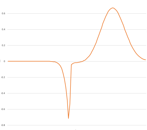
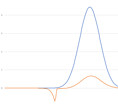
• We can use Markov chains to implement Sample using the Metropolis Algorithm
• If we have a continuous prior (like a mint that produces coins of a certain quality with a certain probability) and a discrete likelihood (like the probability of a coin flip coming up heads), we can use this technique to compute a continuous posterior given an observation of one or more flips.
• This is a very useful technique in many real-world applications.
• Computing the expected value of a distribution given a function is a tricky problem in of itself, but there are a variety of techniques we can use.
• And if we can do that, we can solve some high-dimensional integral calculus problems!

That was rather a lot, and we still did not get to everything I wanted to.

By far the biggest thing that I did not get to, and that I may return to in another series of posts, is: the connection between await as an operator and sampleas an operator  is deeper than you might think.

As I noted above, you can put sample and condition operations in a language and have the compiler build a method that when run, generates a simple, discrete distribution. But it turns out we can actually do a pretty good job of dealing with sample operators on non-discrete distributions as well, by having the compiler be smart about using some of the techniques that we discussed in this series for continuous distributions.

What you really need is the ability to pick a sample, run a little bit of a routine, remember the result, back up a bit and try a different sample, and so on; from this we can build a distribution of program traces, and from that we can build an approximation of the distribution of the output of a probabilistic method!

This kind of control flow is tricky; it’s sort of a generalization of coroutines where you’re allowed to re-run code that you’ve run before, but with different values for the variables to see what happens.

Obviously it is crucially important that the methods be pure! It’s also crucially important that you spend most of your time exploring high-likelihood control flows, because the number of unlikely control flows is nigh infinite. If this sounds a bit like training up an ML model and then using that model in production later, that’s because it is basically the same thing, but applied to programs.

I know what you’re thinking: that sounds bonkers. But —  here is the thing that really got me motivated to write this series in the first place — we actually did it.

A while back my colleague Michael and I hacked together (ha ha) an implementation of multi-shot-continuations for Hack, our PHP variant and showed that we could in fact do probabilistic workflows where we have a distribution, and we sample from it some number of times, and trace out what happens in the program as we do so.

I then went on to work on other projects, but in the meanwhile a team of people who understand statistics far, far better than I do actually built an industrial-strength probabilistic control flow language with a sample operator. 

You can read all about it at their paper Hack PPL: A Universal Probabilistic Programming Language.

Another point that I very much wanted to get to in this series but did not is: we can do the same thing in C#, and in fact we can do it today.

The C# team added the ability to return types other than Task<T> from asynchronous workflows; and it turns out you only need to abuse that feature a small amount to convince C# to “go back a bit” in the workflow – back to the previous await operation, which becomes a stand-in for sample — and re-run portions of it with different sampled values. The C# team could add probabilistic workflows to C# tomorrow.

The C# team has historically done a great job of finding useful monads and embedding them into the control flow of the language; monadic probabilistic workflows with multi-shot continuations could be the next one. How about it team?

Finally, here’s a very incomplete list of papers and web sites that were inspiring to me in writing this series. I learned a lot, and there is plenty more to learn; I’ve just scratched the surface here.

• The idea that we can treat probability distributions like LINQ queries was given to me by my friend and director Erik Meijer; his fun and accessible paper Making Money Using Math hits many of the same points I did in this series, but I did it with a lot more code.
• The design of coroutines in Kotlin was a great inspiration to me; they’ve done a great job of making features that you would normally think of as being part of the language proper, like yield and await, into library methods. The first thing I did in my multi-shot coroutine hack was verify that I could simulate those features. (I was also very pleased to discover that much of this work was implemented by my old colleague Nikov from the C# team!)
• An introduction to probabilistic programming is a book-length work that uses a Lisp-like language with sample and observe primitives.
• Church is another Lisp-like language often used in academic studies of PPLs.
• The webppl.org web site has a Javascript-based implementation of a probabilistic programming language and a lot of great supporting information at dippl.org.

The next few papers are more technical.

• Build Your Own Probability Monads is a good overview for the Haskell programmers out there, as are Practical Probabilistic Programming With Monads and   Stochastic Lambda Calculus and Monads of Probability Distributions.
• Lightweight Implementations of Probabilistic Programming Languages Via Transformational Compilation is a good overview of how you can use MCMC techniques on program traces. A provably correct sampler for probabilistic programs goes into some of the correctness problems faced by PPL implementations, and Generating Efficient MCMC Kernels goes into some of the performance problems.
• Another fascinating area that I wanted to explore in this series is: we know it is bad enough to try to debug programs that have yields and awaits in them; how on earth do you debug programs that are actually running the same code paths maybe thousands of times when exploring the sample space of a workflow? Here’s an interesting paper on debugging probabilistic workflows.

And these are some good ones for the math:

• These MIT course notes on Bayesian updating of continuous priors was a good primer for my episodes on coin flipping. And the lecture notes MC Methods and Importance Sampling are what it says on the tin.
• Understanding the Metropolis-Hastings Algorithm gives a bunch of the underlying math.
• The enormous book Information Theory, Inference and Learning Algorithms was invaluable in getting me up to speed on math I had not done since my undergrad days.

There are many more that I am forgetting, and I’ll add to this list as I recall them.

All right, that was super fun; I am off on my annual vacation where I have no phone or internet, so I’m going to take a bit of a break from blogging; we’ll see you in a month or so for more fabulous adventures in coding!

Let’s sum up the last few episodes:

Suppose we have a distribution of doubles, p, and a function f from double to double. We often want to answer the question “what is the average value of f when it is given samples from p?” This quantity is called the expected value.

The obvious (or “naive”) way to do it is: take a bunch of samples, evaluate the function on those samples, take the average. Easy! However, this can lead to problems if there are “black swans”: values that are rarely sampled, but massively affect the value of the average when run through f. We would like to get a good estimate without having to massively increase the number of samples in our average.

We developed two techniques to estimate the expected value:

First, abandon sampling entirely and do numerical integral calculus:

• Use quadrature to compute two areas: the area under f(x)*p.Weight(x)  and the area under p.Weight(x) (which is the normalization constant of p)
• Their quotient is an extremely accurate estimate of the expected value
• But we have to know what region to do quadrature over.

Second, use importance sampling:

• Find a helper distribution q whose weight is large where f(x)*p.Weight(x) bounds a lot of area.
• Use the naive algorithm to estimate the expected value of  x=>f(x)*p.Weight(x)/q.Weight(x)from samples of q
• That is proportional to the expected value of f with respect to p
• We gave a technique for estimating the proportionality constant by sampling from q also.

The problem with importance sampling then is finding a good q. We discussed some techniques:

• If you know the range, just use a uniform distribution over that range.
• Stretch and shift p so that the transformed PDF doesn’t have a “black swan”, but the normalization constant is the same.
• Use the Metropolis algorithm to generate a helper PDF from Abs(f*p), though in my experiments this worked poorly
• If we know the range of interest, we can use the VEGAS algorithm. It makes cheap, naive estimates of the area of subranges, and then uses that information to gradually refine a piecewise-uniform helper PDF that targets spikes and avoid flat areas of f*p.
• However, the VEGAS algorithm is complex, and I did not attempt to implement it for this series.

The question you may have been asking yourself these past few episodes is:

If quadrature is an accurate and cheap way to estimate the expected value of f over samples from p then why are we even considering doing sampling at all? Surely we typically know at least approximately the range over which f*p has some area. What’s the point of all this?

Quadrature just splits up the range into some number — say, a thousand — equally-sized pieces, evaluates f*p on each of them, and takes the average. That sure seems cheaper and easier than all this mucking around with sampling. Have I just been wasting your time these past few episodes? And why has there been so much research and effort put into finding techniques for estimating expected value?

This series is called “Fixing Random” because the built-in base class library tools we have in C# for representing probabilities are weak. I’ve approached everything in this series from the perspective of “I want to have an object that represents probabilities in my business domain, and I want to use that object to solve my business problems”.

“What is the expected value of this function given this distribution?” is a very natural question to ask when solving business problems that involve probabilities, and as we’ve seen, you can answer that question by simulating integral calculus through quadrature.

But, as I keep on saying: things equal to the same are equal to each other. Flip the script. Suppose our business domain involves solving integral calculus problems. And suppose there is an integral calculus problem that we cannot efficiently solve with quadrature. What do we do?

• We can solve expected value problems with integral calculus techniques such as quadrature.
• We can solve expected value problems with sampling techniques
• Things equal to the same are equal to each other.
• Therefore we can solve integral calculus problems with sampling techniques. 

That is why there has been so much research into computing expected values: the expected value is the area under the function f(x)*p.Weight(x) so if we can compute the expected value by sampling, then we can compute that area and solve the integral calculus problem without doing quadrature!

I said above “if quadrature is accurate and cheap”, but there are many scenarios in which quadrature is not a cheap way to compute an area.

What’s an example? Well, let’s generalize. So far in this series I’ve assumed that f is a Func<double, double> . What if f is a Func<double, double, double> — a function from pairs of doubles to double. That is f is not a line in two dimensions, it is a surface in three.

Let’s suppose we have f being such a function, and we would like to solve a calculus problem: what is the volume under f on the range (0,0) to (1, 1)?

We could do it by quadrature, but remember, in my example we split up the range 0-to-1 into a thousand points. If we do quadrature in two dimensions with the same granularity of 0.001, that’s a million points we have to evaluate and sum. If we only have computational resources to do a thousand points, then we have to have a granularity of around 0.03.

What if the function is zero at most of those points? We could then have a really crappy estimate of the total area because our granularity is so low.

We now reason as follows: take a two-dimensional probability distribution. Let’s say we have the standard continuous uniform implementation of  IWeightedDistribution<(double, double)> .

All the techniques I have explored in this series work equally well in two dimensions as one! So we can use those techniques. Let’s do so:

• What is the estimated value of f when applied to samples from this distribution?
• It is equal to the volume under f(x,y)*p.Weight((x,y)). 
• But p.Weight((x,y)) is always 1.0 on the region we care about; it’s the standard continuous uniform distribution, after all.
• Therefore the estimated expected value of f when evaluated on samples from p is an estimate of the volume we care about.

How does that help?

It doesn’t.

If we’re taking a thousand points by quadrature or a thousand points by sampling from a uniform distribution over the same range, it doesn’t matter. We’re still computing a value at a thousand points and taking an average.

But now here’s the trick.

Suppose we can find a helper distribution q that is large where f(x,y) has a lot of volume and very small where it has little volume.

We can then use importance sampling to compute a more accurate estimate of the desired expected value, and therefore the desired volume, because most of the points we sample from q are in high-volume regions. Our thousand points from q will give us a better estimate!

Now, up the dimensionality further. Suppose we’ve got a function that takes three doubles and goes to double, and we wish to know its hypervolume over (0, 0, 0) to (1, 1, 1).

With quadrature, we’re either doing a billion computations at a granularity of 0.001, or, if we can only afford to do a thousand evaluations, that’s a granularity of 0.1.

Every time we add a dimension, either the cost of our quadrature goes up by a factor of a thousand, or the cost stays the same but the granularity is enormously coarsened.

Oh, but it gets worse.

When you are evaluating the hypervolume of a 3-d surface embedded in 4 dimensions, there are a lot more points where the function can be zero! There is just so much room in high dimensions for stuff to be. The higher the dimensionality gets, the more important it is that you find the spikes and avoid the flats. 

Exercise: Consider an n-dimensional cube of side 1. That thing always has a hypervolume of 1, no matter what n is.

Now consider a concentric n-dimensional cube inside it where the sides are 0.9 long.

• For a 1-dimensional cube — a line — the inner line is 90% of the length of the outer line, so we’ll say that 10% of the length of the outer line is “close to the surface”.
• For a 2-dimensional cube — a square — the inner square has 81% of the area of the outer square, so 19% of the area of the outer square is “close to the surface”.

At what dimensionality is more than 50% of the hypervolume of the outer hypercube “close to the surface”?

Exercise: Now consider an n-dimensional cube of side 1 again, and the concentric n-dimensional sphere. That is, a circle that exactly fits inside a square, a sphere that exactly fits inside a cube, and so on. The radius is 1/2.

• The area of the circle is pi/4 = 79% of the area of the square.
• The volume of the sphere is pi/6 = 52% of the volume of the cube.
• … and so on

At what value for n does the volume of the hypersphere become 1% of the volume of the hypercube?

In high dimensions, any shape that is anywhere on the interior of a hypercube is tiny when compared to the massive hypervolume near the cube’s surface!

That means: if you’re trying to determine the hypervolume bounded by a function that has large values somewhere inside a hypercube, the samples must frequently hit that important region where the values are big. If you spend time “near the edges” where the values are small, you’ll spend >90% of your time sampling irrelevant values.

That’s why importance sampling is so useful, and why we spend so much effort studying how to find distributions that compute expected values. Importance sampling allows us to numerically solve multidimensional integral calculus problems with reasonable compute resources.

Aside: Now you know why I said earlier that I misled you when I said that the VEGAS algorithm was designed to find helpful distributions for importance sampling. The VEGAS algorithm absolutely does that, but that’s not what it was designed to do; it was designed to solve multidimensional integral calculus problems. Finding good helper distributions is how it does its job.

Exercise: Perhaps you can see how we would extend the algorithms we’ve implemented on distributions of doubles to distributions of tuples of doubles; I’m not going to do that in this series; give it a shot and see how it goes!

Next time on FAIC: This has been one of the longest blog series I’ve done, and looking back over the last sixteen years, I have never actually completed any of the really big projects I started: building a script engine, building a Zork implementation, explaining Milner’s paper, and so on. I’m going to complete this one!

There is so much more to say on this topic; people spend their careers studying this stuff. But I’m going to wrap it up in the next couple of episodes by giving some final thoughts, a summary of the work we’ve done, a list of some of the topics I did not cover that I’d hoped to, and a partial bibliography of the papers and other resources that I read when doing this series.

Last time on FAIC we were attacking our final problem in computing the expected value of a function f applied to a set of samples from a distribution p. We discovered that we could sometimes do a “stretch and shift” of p, and then run importance sampling on the stretched distribution; that way we are more likely to sample from “black swan” regions, and therefore the estimated expected value is more likely to be accurate.

However, determining what the parameters to Stretch.Distribution should be to get a good result is not obvious; it seems like we’d want to do what we did: actually look at the graphs and play around with parameters until we get something that looks right.

It seems like there ought to be a way to automate this process to get an accurate estimate of the expected value. Let’s take a step back and review what exactly it is we need from the helper distribution. Start with the things it must have:

• Obviously it must be a weighted distribution of doubles that we can sample from!
• That means that it must have a weight function that is always non-negative.
• And the area under its weight function must be finite, though not necessarily 1.0.

And then the things we want:

• The support of the helper distribution does not have to be exactly support of the p, but it’s nice if it is.
• The helper’s weight function should be large in ranges where f(x) * p.Weight(x) bounds a large area, positive or negative.
• And conversely, it’s helpful if the weight function is small in areas where the area is small.

Well, where is the area likely to be large? Precisely in the places where Abs(f(x)*p.Weight(x)) is large. Where is it likely to be small? Where that quantity is small… so…

why don’t we use that as the weight function for the helper distribution?

Great Scott, why didn’t we think of that before?

Aside: As I noted before in this series, all of these techniques require that the expected value actually exist. I’m sure you can imagine functions where f*p bounds a finite area, so the expected value exists, but abs(f*p) does not bound a finite area, and therefore is not the weight function of a distribution. This technique will probably not work well in those weird cases.

If only we had a way to turn an arbitrary function into a non-normalized distribution we could sample from… oh wait, we do. (Code is here.)

var p = Normal.Distribution(0.75, 0.09);
double f(double x) => Atan(1000 * (x – .45)) * 20 – 31.2;
var m = Metropolis<double>.Distribution(
  x => Abs(f(x) * p.Weight(x)),
  p,
  x => Normal.Distribution(x, 0.15));

Let’s take a look at it:

Console.WriteLine(m.Histogram(0.3, 1));

                         ***            
                         ****           
                        *****           
                       *******          
        *              *******          
       **             *********         
       **             *********         
       **             *********         
       **            ***********        
       **            ***********        
       **           *************       
       **           *************       
      ***           **************      
      ***          ***************      
      ***          ***************      
      ***         *****************     
     ****        *******************    
     ****        ********************   
    *****       *********************** 
----------------------------------------

That sure looks like the distribution we want.

What happens if we try it as the helper distribution in importance sampling? Unfortunately, the results are not so good:

0.11, 0.14, 0.137, 0.126, 0.153, 0.094, ...

Recall that again, the correct result is 0.113. We’re getting worse results with this helper distribution than we did with the original black-swan-susceptible distribution.

I’m not sure what has gone wrong here. I tried experimenting with different proposal distributions and couldn’t find one that gave better results than just using the proposal distribution itself as the helper distribution.

So once again we’ve discovered that there’s some art here; this technique looks like it should work right out of the box, but there’s something that needs tweaking here. Any experts in this area who want to comment on why this didn’t work, please leave comments.

And of course all we’ve done here is pushed the problem off a level; our problem is to find a good helper distribution for this expected value problem, but to do that with Metropolis, we need to find a good proposal distribution for the Metropolis algorithm to consume, so it is not clear that we’ve made much progress here. Sampling efficiently and accurately is hard!

I’ll finish up this topic with a sketch of a rather complicated algorithm called VEGAS; this is an algorithm for solving the problem “how do we generate a good helper distribution for importance sampling knowing only p and f?”

Aside: The statement above is slightly misleading, but we’ll say why in the next episode!

This technique, like quadrature, does require us to have a “range” over which we know that the bulk of the area of f(x)*p.Weight(x) is found. Like our disappointing attempt above, the idea is to find a distribution whose weight function is large where it needs to be, and small where it is not.

I am not an expert on this algorithm by any means, but I can give you a quick sketch of the idea. The first thing we do is divide up our range of interest into some number of equally-sized subranges. On each of those subranges we make a uniform distribution and use it to make an estimate of the area of the function on that subrange.

How do we do that? Remember that the expected value of a function evaluated on samples drawn from a distribution is equal to the area of the function divided by the area of the distribution. We can construct a uniform distribution to have area of 1.0, so the expected value is equal to the area. But we can estimate the expected value by sampling. So we can estimate areas by sampling too! Again: things equal to the same are equal to each other; if we need to find an area, we can find it by sampling to determine an expected value.

So we estimate the expected value of a uniform distribution restricted to each sub-range. Again, here’s the function of interest, f(x)*p.Weight(x)

Ultimately we want to accurately find the area of this thing, but we need a black-swan-free distribution that samples a lot where the area of this thing is big.

Let’s start by making some cheap estimates of the area of subranges. We’ll split this thing up into ten sub-ranges, and do a super cheap estimate of the area of the subrange by sampling over a uniform distribution confined to that subrange.

Let’s suppose our cheap estimate finds the area of each subrange as follows:

Now, you might say, hey, the sum of all of these is an estimate of the area, and that’s what we’re after; and sure, in this case it would be pretty good. But stay focussed: what we’re after here with this technique is a distribution that we can sample from that is likely to have high weight where the area is high.

So what do we do? We now have an estimate of where the area of the function is big — where the expected value of the sub-range is far from zero — and where it is small.

We could just take the absolute value and stitch it all together:

And then use this as our helper distribution; as we prefer, it will be large when the area is likely to be large, and small where it is likely to be small. We’ll spend almost no time sampling from 0.0 to 0.3 where the contribution to the expected value is very small, but lots of time sampling near both the big lumps.

Aside: This is an interesting distribution: it’s a piecewise uniform distribution. We have not shown how to sample from such a distribution in this series, but if you’ve been following along, I’m sure you can see how to do it efficiently; after all, our “unfair die” distribution from way back is basically the same. You can efficiently implement distributions shaped like the above using similar techniques.

This is already pretty good; we’ve done ten cheap area estimates and generated a reasonably high-quality helper PDF that we can then use for importance sampling. But you’ve probably noticed that it is far from perfect; it seems like the subranges on the right side are either way too big or way too small, and this might skew the results.

The insight of the VEGAS algorithm’s designer was: don’t stop now! We have information to refine our helper PDF further.

How?

We started with ten equally-sized subranges. Numbering them from the left, it sure looks like regions 1, 2, 3, 5 and 6 were useless in terms of providing area, and regions 5 and 9 were awesome, so let’s start over with ten unequally sized ranges. We’ll make regions 1, 2, and 3 into one big subrange, and also regions 5 and 6 into one big subrange, and then split up regions 4, 7, 8, 9 and 10 into eight smaller regions and do it again.

Aside: The exact details of how we rebalance the subranges involve a lot of fiddly bookkeeping, and that’s why I don’t want to go there in this series; getting the alias algorithm right was enough work, and this would be more. Maybe in a later series I’ll investigate this algorithm in more detail.

We can then keep on repeating that process until we have a helper PDF that is fine-grained where it needs to be: in the places where the area is large and changing rapidly. And it is then coarse-grained where there is not much change in area and the area is small.

Or, put another way: VEGAS looks for the spikes and the flats, and refines its estimate to be more accurate at the spikes because that’s where the area is at.

And bonus, the helper PDF is always piecewise continuous uniform, which as I noted above, is relatively easy to implement and very cheap to sample from.

This technique really does generate a high-quality helper PDF for importance sampling when given a probability distribution and a function. But, it sounds insanely complicated; why would we bother?

Next time on FAIC: I’ll wrap up this topic with some thoughts on why we have so many techniques for computing expected value.

Last time on FAIC we finally wrote a tiny handful of lines of code to correctly implement importance sampling; if we have a distribution p that we’re sampling from, and a function f that we’re running those samples through, we can compute the expected value of f even if there are “black swan” regions in p. All we need is a helper distribution q that has the same support as p, but no black swans.

Great. How are we going to find that?

A variation on this problem has come up before this series: what should the initial and proposal distributions be when using Metropolis? If we’re using Metropolis to compute a posterior from a prior then we can use the prior as the initial distribution. But it’s not at all clear in general how to choose a high-quality proposal distribution; there’s some art there.

There is also some art in choosing appropriate helper distributions when doing importance sampling. Let’s once again take a look at our “black swan” situation:

As we’ve discussed, I contrived the “black swan” situation by ensuring that there was a region of the graph where the orange line bounded a large area, but the blue line bounded a very tiny area there.

First off: in my initial description of the problem I made the assumption that I only cared about the function on the range of 0.0 to 1.0. If you know ahead of time that there is a specific range of interest, you can always use a uniform distribution over that range as a good guess at a helper distribution. As we saw in a previous episode, doing so here gave good results. Sure, we spend a lot of time sampling a region of low area, but we could tweak that to exclude the region between 0.0 and 0.3.

What if we don’t know the region of interest ahead of time though? What if the PDF and the function we’re evaluating are defined over the whole real line and we’re not sure where to put a uniform distribution? Let’s think about some quick-and-dirty hacks for solving that problem.

What if we “stretched” the blue line a little bit around 0.75, and “squashed” it down a little bit?

The light blue line is not perfect by any means, but we are now likely to get at least a few samples from the part of the orange line that has large negative area.

Since the original distribution is just a normal, we can easily make this helper distribution by increasing the standard deviation. (Code for this episode can be found here.)

var p = Normal.Distribution(0.75, 0.09);
var p2 = Normal.Distribution(0.75, 0.15);
double f(double x) => Atan(1000 * (x – .45)) * 20 – 31.2;
for (int i = 0; i < 10; ++i)
  Console.WriteLine(
    $”{p.ExpectedValueByImportance(f, 1.0, p2):0.###}“);

0.119, 0.114, 0.108, 0.117, 0.116, 0.108, 0.121, ...

Recall that the correct value is 0.113. This is not perfect, but it’s a lot better than the original.

Now, it is all well and good to say that we know how to solve the problem when the nominal distribution is normal; what if it is some arbitrary distribution and we want to “stretch” it?

That’s actually pretty straightforward. Let’s suppose we want to stretch a distribution around a particular center, and, optionally, also move it to the left or right on the real line. Here’s the code:

public sealed class Stretch : IWeightedDistribution<double>
{
  private IWeightedDistribution<double> d;
  private double shift;
  private double stretch;
  public static IWeightedDistribution<double> Distribution(
    IWeightedDistribution<double> d,
    double stretch,
    double shift = 0.0,
    double around = 0.0)
  {
    if (stretch == 1.0 && shift == 0.0) return d;
    return new Stretch(
      d, stretch, shift + around – around * stretch);
  }
  private Stretch(
    IWeightedDistribution<double> d,
    double stretch,
    double shift)
  {
    this.d = d;
    this.stretch = stretch;
    this.shift = shift;
  }
  public double Sample() =>
    d.Sample() * stretch + shift;
  // Dividing the weight by stretch preserves
  // the normalization constant 
  public double Weight(double x) =>
    d.Weight((x – shift) / stretch) / stretch;
}

And now we can get similar results:

var p = Normal.Distribution(0.75, 0.09);
var ps = Stretch.Distribution(p, 2.0, 0, 0.75);
double f(double x) => Atan(1000 * (x – .45)) * 20 – 31.2;
for (int i = 0; i < 10; ++i)
  Console.WriteLine(
    $”{p.ExpectedValueByImportance(f, 1.0, ps):0.###}“);

0.113, 0.117, 0.121, 0.124, 0.12 ...

Again, not perfect, but we’re getting at least reasonable results here.

But like I said before, these are both “more art than science” techniques; they are useful if you have a particular distribution and a particular function, and you’re looking for an expected value, and you’re willing to spend some time writing different programs and trying out different techniques and parameters to tweak it to get good results. We still have not got an algorithm where a distribution and a function go in, and an accurate estimate of the expected value comes out.

Next time on FAIC: I’ll make one more attempt at writing code to get a good result automatically that will fail for reasons I do not know, and sketch out a much more sophisticated algorithm but not implement it.