Let’s take another look at the “hello world” example and think more carefully about what is actually going on:

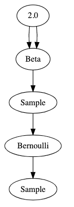
@random_variable
def fairness():
  return Beta(2,2)

@random_variable
def flip(n):
  return Bernoulli(fairness())

heads = tensor(1)
tails = tensor(0)

observations = { flip(0) : heads, ... flip(9): tails }
queries = [ fairness() ]
num_samples = 10000
results = BMGInference().infer(queries, observations, num_samples)
samples = results[fairness()]

There’s a lot going on here. Let’s start by clearing up what the returned values of the random variables are.

It sure looks like fairness() returns an instance of a pytorch object — Beta(2,2) — but the model behaves as though it returned a sample from that distribution in the call to Bernoulli. What’s going on?

The call doesn’t return either. It returns a random variable identifier, which I will abbreviate as RVID. An RVID is essentially a tuple of the original function and all the arguments. (If you think that sounds like a key to a memoization dictionary, you’re right!)

This is an oversimplification, but you can imagine for now that it works like this:

def random_variable(original_function):
  def new_function(*args):   
    return RVID(original_function, args)
  # The actual implementation stashes away useful information
  # and has logic needed for other Bean Machine inference algorithms
  # but for our purposes, pretend it just returns an RVID.
  return new_function

def fairness():
  return Beta(2,2)
fairness = random_variable(fairness)

The decorator lets us manipulate function calls which represent random variables as values! Now it should be clear how

queries = [ fairness() ]

works; what we’re really doing here is

queries = [ RVID(fairness, ()) ]

That clears up how it is that we treat calls to random variables as unique values. What about inference?

Leaving aside the behavior of the decorators to cause random variables to generate RVIDs, our “hello world” program acts just like any other Python program right up to here:

results = BMGInference().infer(queries, observations, num_samples)

Argument queries is a list of RVIDs, and observations is a dictionary mapping RVIDs onto their observed values. Plainly infer causes a miracle to happen: it returns a dictionary mapping each queried RVID onto a tensor of num_samples values that are plausible samples from the distribution of the posterior of the random variable.

Of course it is no miracle. We do the following steps:

• Transform the source code of each queried or observed function (and transitively their callees) into an equivalent program which partially evaluates the model, accumulating a graph as it goes
• Execute the transformed code to accumulate the graph
• Transform the accumulated graph into a valid BMG graph
• Perform inference on the graph in BMG
• Marshal the samples returned into the dictionary data structure expected by the user

Coming up on FAIC: we will look at how we implemented each of those steps.

I’ll get back to Bean Machine and Beanstalk in the next episode; today, a brief diversion to discuss a general principle of language design and congratulate some of my former colleagues.

Back when we were all at Waterloo, a bunch of us were sitting around the comfy lounge, eating C&D donuts and talking about possible future user interfaces for “smart appliances”; this was in the 1990s, long before ubiquitous voice recognition, compute and networking that we take for granted today. I think it was my friend Peter who pointed out that there is a “use vs mention” problem in voice-driven home appliances. We want to be able to mention the toaster in conversation without that causing the toaster to be used.

This was a prescient observation. I have not verified this for myself, but I have heard from reliable sources that in some versions of Amazon’s Alexa smart speaker you could have this conversation:

Human: Alexa, add an item to my to-do list.

Alexa: OK, what do you want to add?

Human: Alexa, what is already on my to-do list?

Alexa: OK, adding Alexa what is already on my to-do list to your to-do list.

(At least the response was not “OK, adding an item to your to-do list”. Thank goodness for small mercies.)

The use-mention distinction is tricky, but I pointed out that you can make at least a little progress by parsing for desires rather than directives. Instead of building a system where we issue a series of commands to our appliances, we could instead give a description of the desired state — I want a pastrami sandwich on toast, no mustard — and let the allegedly smart appliances figure out how to achieve that goal.

(I once told this story to a friend who worked on Alexa; he laughed and pointed out that Alexa is certainly not “smart” and in fact is only barely “obedient”. We have a long way to go.)

This was all on my mind today because the Networked Systems Design and Implementation Symposium has just accepted a paper by some of my Meta colleagues about a declarative domain specific programming language for specifying and achieving desired router states in a datacenter. I reviewed some of their earlier work and made a few small suggestions for improvements to the submission. As a courtesy they listed me as an author; I wish to emphasize that I did none of the actual work whatsoever. 🙂

A huge problem that teams managing datacenters face every day is safely making configuration changes; this is most obvious on days when it goes horribly, horribly wrong. Even if you don’t know anything about router configuration — and I believe packets are moved around the wired network by gnomes and the wireless network by fairies — it’s pretty clear that any time you’re taking a router offline for maintenance or replacement, several things need to happen. You need to have a way to undo the operation back to a known good state if something goes wrong halfway through. You need to move user traffic to another router while still maintaining the ability for administrators to communicate with the target router. And so on. Writing imperative code that ensures that a router whose configuration is changing is always in a controllable state is maybe too easy to get wrong.

Instead, we can take the “I want pastrami on toast” approach. Say what you want to happen under what set of constraints; write a compiler that turns those intentions into an imperative program that you can prove works.

The goal of designing domain-specific languages is to create a language where the problems of the domain are naturally expressed in the jargon of the domain — in this example we can look at the grammar of the language in figure 1 of the paper and immediately see that the language is about describing paths, locations, topologies, routing, propagation, preferences and policies. This pays dividends in understandability of the code by domain experts, and has many other nice benefits.

For example, you can then write a static analyzer which looks for logical errors at the domain level in the code, which is much harder to do with, say, an imperative Python script that makes configuration changes. Even better, the team also has a simulator where they can simulate different network conditions, compile and execute configuration changes, and see if the simulated network is reconfigured as expected; there is no need to “test in production” when making any configuration changes.

Many thanks to the other authors who reached out to me and my manager Walid; I learned a lot from our short collaboration. It is delightful to see an example of a successful, innovative real-world at-scale application of the power of DSLs. Congratulations on being accepted to the symposium!

Next time on FAIC: Back to Bean Machine.

Did I actually build a compiler? Yes and no.

Traditionally we think of a compiler as a program which takes as its input the text of a program written in one language (C#, say), and produces as its output an “equivalent” program written in another language (MSIL, say).  A more modern conception is: a compiler is a collection of code analysis services, and one of those services is translation.

I made a great many assumptions when embarking on this project. Some of the more important ones were as follows:

Assumption: we must implement everything necessary for a source-to-source translation, but that is not enough. The primary use case of Beanstalk is outputting samples from a posterior, not outputting an equivalent program text. Translation may be a secondary use case, but we will not succeed by stopping there.

We’re building a compiler in order to build a better calculator.

Static and dynamic analysis

Traditional translating compilers such as the C# compiler perform a “static” analysis of the code; that is, they analyze only (1) the text of the program and (2) metadata associated with already-compiled artifacts such as libraries. The code is not executed in a static analysis.

“Dynamic” analysis is by contrast an analysis of code while the code is running. 

Assumption: correct static analysis of Python is impossible for at least two reasons. 

1) Python is an extremely dynamic language; it is difficult to definitively know what any program identifier refers to, for example, without actually running the program to find out.

2) The model may depend upon non-stochastic model elements that are unknowable by static analysis. Model parameters or observed values can (and will!) be read from files or queried from databases, and those values must be present in the graph that we deduce.

We must build a dynamic analyzer; we’re going to run a modified version of the model code to find out what it does.

Pure functions, acyclic graph

For our purposes we define a pure function as one that:

• Always terminates normally; it does not go into an infinite loop or throw an exception
• Is idempotent: it always produces the same output when given the same input
• Its action does not depend on mutating global state
• Its action does not mutate global state

Examples of impure functions are easily produced:

mean = 1.0
@random_variable
def normal():
  global mean
  mean = mean + 1.0 # UH OH
  return Normal(mean, 1.0)

Or, just as bad:

mean = tensor([1.0])
@random_variable
def normal():
  global mean
  mean[0] += 1.0
  return Normal(mean, 1.0)

Assumptions:

• Model builders will write pure functions. In particular, model builders will not mutate a tensor “in place” such that the mutation causes a change of behaviour elsewhere in the model
• Beanstalk is not required to detect impure functions, though it may
• Beanstalk may memoize model functions

Also: a Bayesian network never has cycles; the distribution of each node depends solely on the distributions of its ancestor nodes.

Assumptions:

• Model builders will write models where no random variable depends upon itself, directly or indirectly.
• Beanstalk is not required to detect cycles (though in practice, it does)

Note that a model may contain recursion if the recursion terminates. This is legal:

@random_variable
def normal(n):
  if n <= 0:
    mean = 0.0
  else:
    mean = normal(n-1)
  return Normal(mean, 1.0)
queries = [ normal(0) ]
observations = { normal(2): tensor(0.0) }

Next time on FAIC: Having made these and other assumptions, I embarked upon an implementation. But before I can explain the implementation, I should probably answer some nagging questions you might have about what exactly that random_variable decorator does.

Introducing Beanstalk

Last time I introduced Bean Machine Graph, a second implementation of the PPL team’s Bayesian inference algorithm. We can compare and contrast the two implementations:

• BMG emphasizes mechanisms; BMG programs are all about constructing a graph. BM emphasizes business logic
• A point which I did not emphasize yesterday but which will come up again in this series: BMG requires many node constructions be annotated with semantic types like “probability” or “positive real”. BM lacks all “type ceremony”.
• BMG programs represent operations such as addition as verbose calls to node factories. BM concisely represents sums as “x + y ”, logs as “x.log()”, and so on

In short, the BMG user experience is comparatively not a great experience for data scientists, in the same way that writing in machine code is not great for line-of-business programmers. We wished to automatically convert models written in Bean Machine into equivalent programs which constructed a graph, and then got the improved inference performance of BMG.

OK… how?

A program which translates one language to another is called a compiler, and that’s where I came in. We code named the compiler “Beanstalk”. I started working on Beanstalk in October of 2019 given this brief:

Construct a compiler which takes as its input a Bean Machine model, queries and observations, and deduces from it the equivalent BMG graph (if there is one).

If we can solve that problem effectively then we get the best of both worlds. Data scientist users can write models using a pleasant Python syntax easily integrated into their existing PyTorch workflows, but get the inference performance afforded by BMG. The “concept count” — the number of APIs that the data scientist must understand — increases only slightly, but their workflows get faster. That is a win all around.

Does it work today?

Yes. Barely. If for some strange reason you want to play around with it, you can obtain the code from github. The error messages are terrible, the compiler is “over fit” to specific models that we needed to get compiled, and it is quite slow, but for simple models it does work. At the time the team was shut down we were actively extending both BMG and the compiler to handle more general models efficiently.

Early on we realized that of course the compiler is a means to an end, not an end in itself. What users really wanted was a more efficient inference engine that just happened to use BMG as its back end, so that’s the main API. You can call BMGInference().infer(), passing in queries, observations, and so on, just like any other Bean Machine inference engine; the compiler will analyze the source code of the queries, produce a graph, and call BMG’s inference engine to produce samples from the queries posteriors.

It has a few other useful APIs as well that are more like a traditional source-in-source-out compiler.

• BMGInference().to_graph() produces a graph object without starting inference.
• BMGInference().to_python() and to_cpp() produce Python and C++ source code fragments which construct the graph.
• BMGInference().to_dot() produces a program in the DOT graph visualization language; that’s what I used to make the graph diagrams in this series.

Next time on FAIC: What were my initial assumptions when tasked with writing a “compiler” that extracts a graph from the source code of a model? And is it really a compiler, or is it something else?

Introducing Bean Machine Graph

Bean Machine has many nice properties:

• It is integrated with Python, a language often used by data scientists
• It describes models using the rich, flexible pytorch library
• Inference works well even on models where data is stored in large tensors

I’m not going to go into details of how Bean Machine proper implements inference, at least not at this time. Suffice to say that the implementation of the inference algorithms is also in Python using PyTorch; for a Python program it is pretty fast, but it is still a Python program.

We realized early on that we could get order-of-magnitude better inference performance than Bean Machine’s Python implementation if we could restrict values in models to (mostly) single-value tensors and a limited set of distributions and operators.

In order to more rapidly run inference on this set of models, former team member Nim Arora developed a prototype of Bean Machine Graph (BMG).

BMG is a graph-building API (written in C++ with Python bindings) that allows the user to specify model elements as nodes in a graph, and relationships as directed edges. Recall that our “hello world” example from last time was:

@random_variable
def fairness():
  return Beta(2,2)

@random_variable
def flip(n):
  return Bernoulli(fairness())

That model written in BMG’s Python bindings would look like this: (I’ve omitted the queries and observations steps for now, and we’ll only generate one sample coin flip instead of ten as in the previous example, to make the graph easier to read.)

g = Graph()
two = g.add_constant_pos_real(2.0)
beta = g.add_distribution(
  DistributionType.BETA,
  AtomicType.PROBABILITY,
  [two, two])
betasamp = g.add_operator(OperatorType.SAMPLE, [beta])
bern = g.add_distribution(
  DistributionType.BERNOULLI,
  AtomicType.BOOLEAN,
  [betasamp])
flip0 = g.add_operator(OperatorType.SAMPLE, [bern])

That’s pretty hard to read. Here’s a visualization of the graph that this code generates:

These graphs are properly called Bayesian network diagrams, but for this series I’m just going to call them “graphs”.

I should say a little about the conventions we use in this graphical representation. Compiler developers like me are used to decomposing programs into abstract syntax trees. An AST is, as the name suggests, a tree. ASTs are typically drawn with the “root” at the top of the page, arrows point down, “parent nodes” are above “child nodes”, and operators are parents of their operands. The AST for something like x = a + b * c would be

where X, A, B, C are identifier nodes.

Bayesian network diagrams are just different enough to be confusing to the compiler developer. First of all, they are directed acyclic graphs, not trees. Second, the convention is that operators are children of their operands, not parents.

The best way I’ve found to think about it is that graphs show data flow from top to bottom. The parameter 2.0 flows into an operator which produces a beta distribution — twice. That distribution flows into a sample operator which then produces a sample from its parent distribution. That sampled value flows into an operator which produces a Bernoulli distribution, and finally we get a sample from that distribution.

If we wanted multiple flips of the same coin, as in the original Python example, we would produce multiple sample nodes out of the Bernoulli distribution.

BMG also has the ability to mark sample nodes as “observed” and to mark operator nodes as “queried”; it implements multiple inference algorithms which, just like Bean Machine proper, produce plausible samples from the posterior distributions of the queried nodes given the values of the observed nodes. For the subset of models that can be represented in BMG, the performance of the inference algorithms can be some orders of magnitude faster than the Bean Machine Python implementation.

Summing up: Our team had two independent implementations of inference algorithms; Bean Machine proper takes as its input some decorated Python methods which concisely and elegantly represents models in a highly general way using PyTorch, but the inference is relatively slow. Bean Machine Graph requires the user to write ugly, verbose graph construction code and greatly restricts both the data types and the set of supported operators, but uses those restrictions to achieve large inference speed improvements.

Next time on FAIC: Given the above description, surely you’ve guessed by now what the compiler guy has been doing for the last three years on this team full of data scientists! Can we automatically translate a Bean Machine Python model into a BMG graph to get BMG inference performance without sacrificing representational power?

As I mentioned in the previous episode, the entire Bean Machine team was dissolved; some team members were simply fired, others were absorbed into other teams, and some left the company. In this series I’m going to talk a bit about Bean Machine and my work on what is surely the strangest compiler I’ve ever written.

I should probably recap here my introduction to Bean Machine from what now seems like an eternity ago but was in fact only September of 2020.

We also have some tutorials and examples at beanmachine.org, and the source code is at github.com/facebookresearch/beanmachine.

We typically think of a programming language as a tool for implementing applications and components: games, compilers, utilities, spreadsheets, web servers, libraries, whatever. Bean Machine is not that; it is a calculator that solves a particular class of math problems; the problems are expressed as programs.

The purpose of Bean Machine is to allow data scientists to write declarative code inside Python scripts which represents relationships between parts of a statistical model, thereby defining a prior distribution. The scientist can then input real-world observations of some of the random variables, and queries on the posterior distributions. That is, we wish to give a principled, mathematically sound answer to the question: how should we update our beliefs when given real-world observations?

Bean Machine is implemented as some function decorators which modify the behavior of Python programs and some inference engines which do the math. However, the modifications to Python function call semantics caused by the decorators are severe enough that it is reasonable to conceptualize Bean Machine as a domain specific language embedded in Python.

The “hello world” of Bean Machine is: we have a mint which produces a single coin; our prior assumption is that the fairness of the coin is distributed somehow; let’s suppose we have reason to believe that it is drawn from beta(2,2).

@random_variable
def fairness():
  return Beta(2,2)

We then flip that coin n times; each time we call flip with a different argument represents a different coin flip:

@random_variable
def flip(n):
  return Bernoulli(fairness())

We then choose an inference algorithm — say, single-site Metropolis — say what we observed some coin flips to be, and ask for samples from the posterior distribution of the fairness of the coin. After all, we have much more information about the fairness of the coin after observing some coin flips than we did before.

heads = tensor(1)
tails = tensor(0)
samples = bm.SingleSiteAncestralMetropolisHastings().infer(
    queries=[fairness()],
    # Say these are nine heads out of ten, for example.
    observations={ flip(0) : heads, [...] flip(9): tails },
    num_samples=10000,
    num_chains=1,
)

If we then did a histogram of the prior and the posterior of fairness given these observations, we’d discover that as the number of samples increased, the histograms would conform more and more closely to these graphs:

Prior: Beta(2,2)

Posterior if we got nine heads and one tail in the observations:

When we observe nine heads out of ten, we should update our beliefs about the fairness of the coin by quite a large amount.

I want to emphasize that what this analysis gives you is not just a point estimate — the peak of the distribution — but a real sense of how tight that estimate is. If we had to make a single guess as to the fairness of the coin prior to observations, our best guess would be 0.5. In the posterior our best guess would be around 0.83. But we get so much more information out of the distribution! We know from the graphs that the prior is extremely “loose”; sure, 0.5 is our best guess, but 0.3 would be entirely reasonable. The posterior is much tighter. And as we observed more and more coin flips, that posterior would get even tighter around the true value of the fairness.

Notice also that the point estimate of the posterior is not 0.9 even though we saw nine heads out of ten! Our prior is that the coin is slightly more likely to be 0.8 fair than 0.9 fair, and that information is represented in the posterior distribution.

All right, that’s enough recap. Next time on FAIC: I’m not going to go through all the tutorials on the web site showing how to use Bean Machine to build more complex models; see the web site for those details. Rather, I’m going to spend the rest of this series talking about my work as the “compiler guy” on a team full of data scientists who understand the math much better than I do.