Source code for this episode is here.

Just as a reminder: I am developing my C# version of Stafford’s “QLIFE” algorithm by taking Abrash’s “keep the neighbour counts around” algorithm and gradually adding optimizations. That’s much easier to understand than trying to explain the whole complicated thing at once.

So far, we’ve got the following algorithm:

• Keep up-to-date neighbour counts of all cells in a byte array
• Maintain a list of cells which changed on the previous tick
• On the current tick, examine only the cells which changed on the previous tick and their neighbours. Update the ones that changed, and create a deduplicated change list for the next tick.

However, we are still using a similar technique as we used in our naïve algorithm to ensure that we never write a cell before we need to read its value: we make a complete copy of all the cells on each tick, read from the copy, and write to the original. Making that copy is fast, but it is O(n) in the total number of cells; it seems plausible that we ought to be able to come up with an algorithm that is O(changed cells).

Here’s what we’re going to do.

Recall that we are spending one byte per cell, but are only using five of the eight bits available in a byte: four for the neighbour count, one for the state. We’re going to use one of the extra bits to store the next state of a cell that is about to change.

Why do we need that? Surely if we already know what cells are about to change, then the next state is just the opposite of the current state, right? But we need it because we are trying to solve two problems at once here: compute the new state, and deduplicate the new change list without using a hash table. Since we are looking at all neighbours of previously-changed cells, we will frequently end up looking at the same cells multiple times, but we do not want the change list to become more and more full of duplicates as time goes on. If the “next state” and the “current state” bits are the same, then we already updated the current state, so we can skip adding it to the new change list, and thereby deduplicate it. (As I noted last time, we’ll get to algorithms that use automatically-deduplicated sets in future episodes.)

As always I want the bit twiddling to be isolated into methods of their own and structs to be immutable. Adding accessors for another bit in my Cell struct is straightforward:

private const int next = 5;
private const int nextm = 1 << next;
public bool Next => (cell & nextm) != 0;
public Cell NextAlive() => new Cell((byte)(cell | nextm));
public Cell NextDead() => new Cell((byte)(cell & ~nextm));

Easy peasy. I’m going to change the Step algorithm but everything else — BecomeAlive and BecomeDead in particular — stays exactly the same. As does most of Step:

public void Step()
{

We’re going to create a new, temporary list of the cells that are about to change on this tick. This list is allowed to have duplicates.

  var currentChanges = new List<(int, int)>();

There is a line of code conspicuous by its absence here. We are not cloning the array!

Once again we loop over the cells which changed last time and their neighbours; this is all the same:

  foreach ((int cx, int cy) in changes)
  {
    int minx = Max(cx - 1, 1);
    int maxx = Min(cx + 2, width - 1);
    int miny = Max(cy - 1, 1);
    int maxy = Min(cy + 2, height - 1);
    for (int y = miny; y < maxy; y += 1)
    {
      for (int x = minx; x < maxx; x += 1)
      {

Once again we have the Life condition that you are now familiar with:

        Cell cell = cells[x, y];
        int count = cell.Count;
        bool state = cell.State;
        bool newState = count == 3 | count == 2 & state;

Is this cell going to change? If so, record the new state in bit 5 and add it to the current changes list:

        if (state & !newState)
        {
          currentChanges.Add((x, y));
          cells[x, y] = cell.NextDead();
        }
        else if (!state & newState)
        {
          currentChanges.Add((x, y));
          cells[x, y] = cell.NextAlive();
        }
      }
    }
  }

Again, yes, I could do the mutation of the bit in-places since we have a collection of variables, but I can’t bring myself to mutate a value type.

We’re done our first pass; the list of previous changes is now useless to us:

  changes.Clear();

The second pass is much simpler than the first. For all the cells that need changing, use idempotent helper functions from last time to record the new neighbour counts and update the change list for the next tick:

  foreach ((int x, int y) in currentChanges)
  {
    if (cells[x, y].Next)
      BecomeAlive(x, y);
    else
      BecomeDead(x, y);
  }
}

And we’re done.

If you look at the asymptotic performance, plainly it is O(changed cells), and not O(total number of cells), which is great! This means that we could have extremely large boards with lots of empty space or still lifes, and we only pay a per-tick time price for the evolving or oscillating cells that change.

Our “static” memory consumption, for the array, is still O(total cells) of course, but our dynamic burden on the garbage collector is also O(changed cells) per tick, which seems like it ought to be a win.

What about our actual performance of computing acorn for 5000 cycles on an 8-quad?

Algorithm           time(ms)  ticks  size(quad)    megacells/s
Naïve (Optimized):   4000       5K      8               82
Scholes              3250       5K      8              101  
Frijters SIMD        1000       5M      4             1200
Abrash                550       5K      8              596
Abrash w/ changes     190       5K      8             1725 
Abrash, O(c)          240       5K      8             1365

I was slightly surprised to discover that it is around 20% slower! As I have pointed out a number of times, copying a 64K array of bytes is astonishingly fast. That’s the thing to always remember about asymptotic performance: it is about how the performance cost changes as the problem becomes large. It would be interesting to do some scaling experiments and discover when the cost of copying the array becomes the dominating cost, but I’m not going to; if anyone wants to do the experiment please do and report back.

Update: Reader jaloopa has done the experiment on their machine; when bumping up from an 8-quad to a 10-quad — so, just 16 times bigger — the O(c) algorithm is ten times faster than the O(n) algorithm! So this is actually a big win once the board sizes get significantly larger than 64KB. I was closer to the break-even point than I thought.

Next time on FAIC: I’ve been talking a lot about Life algorithms but very little about Life itself. Let’s digress for an episode or two and explore some interesting basic patterns.

After that: We are now using six bits per cell to store the neighbour count, current state and next state. If we can get that back down to five bits per cell then we can fit three cells into a two-byte short. That’s slightly more memory efficient, but at a cost of greatly increasing the amount of bit twiddling we need to do. This seems like a performance-killing change; will it eventually pay for itself by enabling further optimizations, or is it a big waste of effort? We’ll find out!

Code for this episode can be found here. Exciting news for the client; I have added a play/pause button. I suppose I could have added that single line of code earlier, but hey, better now than later.

Last time on FAIC I presented a Life algorithm from an early 1990s article in PC Techniques magazine by noted optimization guru Michael Abrash; the basic idea was to observe that we can add redundancy by storing the current neighbour count of every cell in the cell itself. The added cost of having to update that redundant data infrequently more than pays for the cost of having to not recompute it frequently.

The sequel to that article, which is available as chapter 18 of the book I mentioned last time, gives a nigh-impenetrable account of improvements to Abrash’s algorithm made by David Stafford. There are a number of pedagogic problems with the way the algorithm is presented; what I’ve settled on is to do a series of episodes where I gradually mutate Abrash’s algorithm into Stafford’s. Today we’ll start with a “change list” optimization.

I noted at the end of the last episode that the algorithm “knows what changed”, and that should have got your optimization sense tingling. That is information we can use provided that we can keep it around! The key observation to make here is:

If a cell did not change on the previous tick, and also none of its neighbours changed on the previous tick, then the cell will not change on the next tick.

But that is phrased with too many negatives; let’s turn that into a positive statement:

The only cells which might change on the next tick are those that changed on the previous tick, or the neighbour of a cell that changed on a previous tick.

If you are not convinced that first, both statements are equivalent, and second, that they are both correct, make sure you are able to convince yourself before reading on, because this is the key observation that we need to make this optimization.

What we can do then is update our existing implementation of the “store the counts in the cells” algorithm to remember what cells changed on the previous tick. On the next tick, instead of looping over every cell in the grid, we loop over the cells which changed previously, and the neighbors of those cells.

Now before I write the code, I am sure that the attentive readers have immediately noticed a problem. What if two near to each other cells both changed on the previous tick?  They might share up to four neighbors, and so it sounds like we might be recomputing those neighbours potentially multiple times. This could have a performance impact, because we are doing unnecessarily duplicated work, and worse, it could have a correctness impact.

What is the correctness impact? Remember that the key to Abrash’s algorithm is that we maintain the invariant that the redundantly stored neighbour count is accurate. Our implementation had the property that every cell was considered once, and so if it changed, it updated the neighbour counts once. What if that is no longer the case? You can imagine a scenario where we say “OK, this cell is becoming alive so increment all the neighbour counts”, and then we do that a second time and now the neighbour counts are disastrously wrong.

There are two ways to deal with this situation:

• Somehow detect the “I’ve got two changes that have neighbors in common” situation to deduplicate the “possibly affected neighbours” set. This then involves additional data structures and additional work, all of which is solely in the service of maintaining consistency of a redundant data structure. Redundancy has costs!
• Make updates idempotent. A second update becomes a no-op. If your “I’ve done this already” check is fast then the performance impact of “doing the same work twice” becomes minimal.

In modern C# code where I have debugged and fast generic set and dictionary classes available instantly I would be inclined to use the first approach — and indeed, we will make heavy use of such classes in later episodes. But in keeping with the spirit of the original 1990s-era implementations written in simple C or assembler, I’m going to for now stick with the second approach and just use a simple algorithm. As we will see, if we are clever we can get a deduplicated “recent changes” list for free, even if we end up touching some neighbouring cells twice.

In x86 assembler you would not even have a list data type; you’d just grab a block of memory to store cell pointers and keep a “high water mark” to the current top of the list. But to make this somewhat more accessible to the modern C# programmer we’ll make a list of tuples; the algorithm is basically the same regardless of the implementation of the list.

The cell definition will be exactly the same, so I will not repeat that.  We keep one extra piece of state, which is “what changed on the last tick?”

        private List<(int, int)> changes;

Oh my goodness how I love finally having tuples in C#. How did we ever live, having to build little structs for these trivial tasks?

The BecomeAlive and BecomeDead helpers are the same except for two small changes. First, they are now idempotent, and second, they record when they got a change:

private void BecomeAlive(int x, int y)
{
  if (cells[x, y].State)
    return; // Already became alive; cheap idempotency!
  changes.Add((x, y));
  // ... and the rest is the same ...

Since the only place we add to the new change list is here, and since these methods are now idempotent, the change list for next time will be deduplicated.

We make some minor changes to the step function to ensure that we are iterating over only valid neighbours of recently-changed points, and we are saving the locations of the newly-changed points:

public void Step()
{
  Cell[,] clone = (Cell[,])cells.Clone();
  var previousChanges = changes;
  changes = new List<(int, int)>();
  foreach((int cx, int cy ) in previousChanges)
  {
    int minx = Max(cx - 1, 1);
    int maxx = Min(cx + 2, width - 1);
    int miny = Max(cy - 1, 1);
    int maxy = Min(cy + 2, height - 1);
    for (int y = miny; y < maxy; y += 1)
    {
      for (int x = minx; x < maxx; x += 1)
      {
        Cell cell = clone[x, y];
        int count = cell.Count;
        if (cell.State)
        {
          if (count != 2 && count != 3)
            BecomeDead(x, y);
        }
        else if (count == 3)
          BecomeAlive(x, y);
      }
    }
  }
}

I’ve also removed the “is this cell and all its neighbours dead?” check. Why? Because now that we are only looking at changed cells and their neighbours, the “dead cell in the middle of eight dead cells” case is now rarely processed in the inner loop. Remember, the whole idea of this optimization was to identify regions of the board that are changing, and isolated dead cells are not changing.

Put another way: to be in that situation in this algorithm, the cell under consideration must have either (1) been a living cell with no living neighbours, which is rare, or (2) been a cell who had living neighbours which all died, which is also rare.

What are the performance characteristics of this algorithm with the change tracking optimization?

First off, it is still O(n) in the number of cells in both time and memory because of that pesky array clone in there. What about the new costs that we’ve added? Maintaining the change list is O(number of changes) in both time and space, and the number of changed cells is always less than the number of cells, so this additional burden cannot be worse than O(n).

What about the raw speed?

Algorithm           time(ms)  ticks  size(quad)    megacells/s
Naïve (Optimized):   4000       5K      8               82
Scholes              3250       5K      8              101  
Frijters SIMD        1000       5M      4             1200
Abrash                550       5K      8              596
Abrash w/ changes     190       5K      8             1725 

We have a new winner once again, at almost three times the throughput of our previous version, and beating the (unscalable) SIMD 16×16 implementation in cells per second. This is over 20x faster than our minimally-optimized naive version!

That pesky array allocation sure is irritating, isn’t it? That right now is the only thing keeping us from making this algorithm O(changes) in time instead of O(n). It seems like we could have an algorithm where no matter how big the board was, the time cost of computing a new board would be proportional to the number of cells which changed, and not the number of cells overall.

Next time on FAIC: that seems like an attractive property for an algorithm to have, so let’s make it happen!

Source code for this episode is here. I’ve added a panel to the UI that moves as the UI is resized; I’ll add some controls to it in future episodes.

Back in 1994 I made a photocopy of an article from the January issue of PC Techniques magazine; it was about the winner of a Life optimization contest for x86 programmers, and the algorithm in it was, and still is, nigh impenetrable. We will attempt to penetrate some of its secrets later on in this series. Back in 1994 I put it in my file folder of articles about Life to come back to later and then I did not for, well, I guess for 26 years. Where does the time go?

The article was the second of a series of three, and I always meant to look up the other two but never did. I believe the third was never written, but I was pleasantly astonished when researching this series to discover that the first two articles were not only available on the internet, but the markup source code of the articles is checked in to GitHub. You can read the two articles — not in markup — here; they have been reformatted into chapters of a book about optimization. I look forward to reading the whole thing; it looks fascinating.

They are long articles with lots of source code, so don’t worry if you don’t want to read it all; I’ll summarize the key points here and provide my own C# implementation of the algorithm described.

I never met Michael Abrash when I was at Microsoft, but of course he was well known as an optimization guru. Reading chapter 17 of this book now, 25 years later, I am powerfully struck by what is dated and what is timeless.

Of course the hardware details are extremely dated. In 1994 DOOM ran at a resolution of 320×200; a 200×200 Life board was considered large. The target machine for achieving acceptable performance in Abrash’s Life optimization was a 20MHz 486. A mere 26 years later I’m typing this on a mid-range 12 core 3.2GHz i7 with two 1920×1080 monitors, and (leaving aside Jeroen’s fun 16×16 proof-of-concept adventure) I would consider any Life grid of less than 256×256 at a bare minimum to be unreasonably small. Kids today don’t know how good they have it and should get off my lawn.

Similarly, “kids today” reading Abrash’s article might wonder why on Earth he is so concerned about “segments”, whatever those are; I encourage you to read up on segmented memory architectures and just imagine how much fun it is to live in a world where there are pointers of different sizes for different-sized allocations. A uniform 64 bit process-isolated virtual address space is a dream come true.

The seemingly very dated part though is the notion that writing a program in hand-optimized assembly is crucial for truly achieving maximum performance. The basic idea here is that humans know how to beat the compiler at its own game of translating their algorithms into optimized assembly.

Though undoubtedly there are still a few tricks and tips that assembly language experts can pull off from time to time, we are all better off with the attitude that if there’s a way to identify a pattern and wring some extra performance out of an optimization, then put that pattern in the compiler’s optimization pass. That way we all get it.

I want to be clear here that Abrash was absolutely correct in 1994. I could tell war stories; for example, in 1996 there was a bug in the MSVC compiler where it would de-optimize certain switch statements, and since the inner loop of the JScript engine was a switch statement over the bytecode opcodes, this was a major regression in script engine performance. When the VC team could not promise that they’d fix the bug before we shipped, we ended up writing a bunch of macros and assembler that re-optimized the switch statement. There were many other examples of code in Visual Basic, VBScript, JScript, OLE Automation, and other key components where we’d call into little hand-optimized assembly routines when the compiler couldn’t do a good enough job to meet our needs. When the Excel inner loop was rewritten from hand-optimized assembly into C, that was a big deal. And so on.

Why did I say seemingly above? Because this actually is not dated if we look at it more generally.

I’m sure that over reading this series, many readers have said to themselves “oh, I see how to improve this, let’s rewrite it in unsafe C# and use pointers to avoid memory safety checks…” Inline assembly is to C as unsafe code is to C#. Both are the ability to say “the relatively safe abstractions afforded by this language are preventing me from accessing the performance capabilities of the underlying unsafe implementation”. By taking the burden on ourselves of guaranteeing safety instead of relying on the compiler or runtime, we can bypass some safety checks that we “know” to be unnecessary. The problems arise, of course, when we are wrong!

But what I love about reading this article 26 years after I first intended to is seeing how much of that 1990s Microsoft performance culture I’ve internalized and how much is still relevant today:

• The underlying theme of this series: find the characteristics of your problem space that admit optimizations, rather than relying on improving raw speed at the margins.
• Get the algorithmic complexity understood first before you try to optimize, particularly if scaling is important.
• Know your target; what are the capabilities of the user’s hardware? What performance metrics are relevant to them? Don’t optimize the wrong thing, and don’t optimize for hardware no user has.
• Measure. Profile. Attack the biggest problem, and then measure again.
• Listen to your intuitions but be prepared to be proven wrong wrong wrong.
• Choosing the wrong abstraction can make it difficult to reason about performance and fix performance problems.
• You can often trade off between space and time; if you can afford more space then you can achieve less time, though beware of the fact that it takes time to fill that space.
• You can often trade off between generality and performance; sometimes you can solve a more restricted problem much faster. But even better, sometimes you can realize that a generalization leads you to a faster solution through an algorithmic improvement.
• Heavily optimized programs are confusing, hard to read, and hard to change, and hard to make even faster. Always try to make it right, then make it clear, and only then try to make it fast. A fast program that is wrong or is unclear, is just making future work harder.

I’m not going to take all of this advice in this series — I optimize plenty of stuff in my day job! — but it is a good summary of the sorts of things I want to keep in mind as we proceed with the next few episodes.

Aside: A commenter asked me in the previous episode what the point of all this optimization is; normally of course I am all about “know what metrics are important to your customer and measure those”, but I haven’t said what the goal state is other than “bigger and faster please”. That’s a great point and I should address it in a future episode; why exactly do we want to compute really large Life boards really fast? But the short answer is: there are interesting structures that have millions of living cells and take hundreds of thousands of ticks to run, and we cannot effectively explore those structures if the client is restricted to an 8-quad. More on this later!

Enough chitchat and reminiscing; what were Abrash’s observations of Life characteristics that lead us towards an improved algorithm?

• Because of the overcrowding rule, it is impossible for a majority of cells to be alive.
  • I already observed this fact in an early episode when I pointed out that my display abstraction is “call me back with the locations of all the living cells in this grid subset”, but it is good to bring it up again because it is a key point in many Life algorithms.
  • In fact, the most common kind of dead cell is the isolated dead cell — a dead cell surrounded by eight other dead cells.
• If you watch a pattern like acorn run for a while you see that there are three kinds of living cells:
  • The majority of living cells are in “still lifes” — ponds, beehives, and so on.
  • There are very small number of cells in oscillators and gliders that change consistently.
  • Then there are one or more “fronts” of destruction and creation as changing patterns overlap the still lifes and oscillators.
• The naive algorithm spends most of its time counting living neighbours.
• Still lifes away from the “fronts” and isolated dead cells do not change their neighbour counts from one tick to the next.

The most basic conclusion we can draw from these observations is: we could trade space off for time and store the neighbour counts along with the cell state; they almost never change, and if they don’t change, we don’t need to recompute them.

Moreover, we don’t even need to make a space tradeoff because I already had been using one byte per cell! In two previous episodes I discussed doing a computation where we add up a cell and all the living neighbours and then add on top of that the original cell multiplied by 8. But we could simply have a small variation on  that as our basic data structure. We’ll declare that a cell is a byte where bits 0 through 3 are the neighbour count, and bit 4 is the state of the cell.

I like to start by making a thin abstraction over bytes that gives me the semantics I want. Those semantics are: current state, current neighbor count, increase and decrease the count:

struct Cell
{
  private readonly byte cell;
  public Cell(byte cell)
  {
    this.cell = cell;
  }
  private const int state = 4;
  private const int statem = 1 << state;
  private const int countm = 0xf;
  public bool State => (cell & statem) != 0;
  public int Count => cell & countm;
  public bool AllDead => cell == 0;
  public Cell MakeAlive() => new Cell((byte)(cell | statem));
  public Cell MakeDead() => new Cell((byte)(cell & ~statem));
  public Cell Increment() => new Cell((byte)(cell + 1));
  public Cell Decrement() => new Cell((byte)(cell - 1));
  }
}

Long time readers will surely know that I always want the bit twiddling to be out of the mainline code and in helper methods where it is nicely hidden. The jitter will, we hope, do a good job of inlining these operations.

Mutable structs are of course pure evil; even though we’re going to be using an array of these things and the array is a collection of mutable variables, so there would be no problem mutating a struct, I just can’t bring myself to do it.

We will go back to our naive algorithm roots and declare a two-d array of cells as our grid: (I’m skipping over the boring boilerplate; see the GItHub source code for details if you want it; I’ve also omitted the debug assertions and comments and whatnot.)

class Abrash : ILife
{
  private const int height = 258;
  private const int width = 258;
  private Cell[,] cells;

We now have a bunch of work to do every time a cell becomes alive that was dead, or a cell dies that was alive; namely, the neighbour counts of its eight neighbours is now wrong. Let’s make a couple methods to help out with that. First, one that makes a dead cell become alive:

private void BecomeAlive(long x, long y)
{
  // Make a dead cell come alive.
  cells[x - 1, y - 1] = cells[x - 1, y - 1].Increment();
  cells[x - 1, y] = cells[x - 1, y].Increment();
  cells[x - 1, y + 1] = cells[x - 1, y + 1].Increment();
  cells[x, y - 1] = cells[x, y - 1].Increment();
  cells[x, y] = cells[x, y].MakeAlive();
  cells[x, y + 1] = cells[x, y + 1].Increment();
  cells[x + 1, y - 1] = cells[x + 1, y - 1].Increment();
  cells[x + 1, y] = cells[x + 1, y].Increment();
  cells[x + 1, y + 1] = cells[x + 1, y + 1].Increment();
}

And I won’t bore you with BecomeDead; it’s just the same but in the other direction.

Of course we still must ensure that we do not mutate the array as we are iterating over it, so let’s once again go back to our pre-naive-optimization days and just make a copy of the current state; we’ll iterate over the copy and use it to decide how to mutate the current state array. The algorithm is very straightforward:

public void Step()
{
  Cell[,] clone = (Cell[,])cells.Clone();
  for (int y = 1; y < height - 1; y += 1)
  {
    for (int x = 1; x < width - 1; x += 1)
    {
      Cell cell = clone[x, y];
      if (cell.AllDead)
        continue;
      int count = cell.Count;
      if (cell.State)
      {
        if (count != 2 && count != 3)
          BecomeDead(x, y);
      }
      else if (count == 3)
        BecomeAlive(x, y);
    }
  }
}

Notice that unlike Abrash’s implementation, I am not doing “wrap around” semantics. Rather, I’m never updating the edges; they will stay dead forever. This means that we can entirely skip doing any validity checking when updating neighbours, because every cell that can change has eight good neighbours.

However, I also bumped up the grid size to 258×258, so that we are still computing an entire 8-quad worth of cells. We can live with wasting a KB of memory here. (Of course back in the days of writing hand-optimized 80486 assembler it would be unattractive to bump up past a 64 KB buffer because now you need a long pointer to address all of it, and have I mentioned that I am glad to no longer have to remember the rules for segmented architectures?)

I’m doing this mostly to keep the code simple, but by not checking the edge conditions in theory we ought to get a slight speed improvement. However, recall that when I attempted the same “optimization” on the naïve algorithm, performance got very slightly worse so things are maybe not as easy to analyze as I’m making out here.

The “continue the loop if the cell is an isolated dead cell” check is not strictly speaking necessary; the algorithm is correct without it. But there are two things here. First, as I mentioned before, this is the common easy out. Dead cells with all dead neighbours is the most common case, and it is the cheapest to check, so check it as soon as possible so you can skip on to the next loop iteration.

Second, in Abrash’s original implementation, the operation “skip ahead in this loop over an array to the first non-zero byte” can be fairly easily identified by an optimizing C compiler and turned into a single x86 machine instruction; this optimization was common in optimizing compilers of that age and I mentioned a related optimization it in a previous episode. (The optimization is apparently no longer a win on modern hardware.)

What is the asymptotic complexity of this algorithm? Give that some thought and then scroll down.

.

.

.

.

.

.

.

.

If the number of cells in the grid is n, then we clone an array, which is O(n) cost. Then we do O(n) loop counter operations and O(n) comparisons to zero per step. The algorithm has to be at least O(n), and in fact it is O(n) still, in both time and space.

However, we can be a little bit more sophisticated here and notice that though there are always n operations total inside the loop, we can divide them into three buckets:

• Extremely cheap operations: continue if equal to zero is one of the cheapest things you can put into a loop. Since most cells are typically isolated dead cells, most cells fall into this bucket.
• Very cheap operations: fetch the state and the count, do some comparisons on them, and discover that the cell does not need to change. We do a little more work here, but of the cells which are not isolated dead cells, most of them are unchanging cells in a typical Life instance.
• Comparatively expensive operations: change a cell, update the eight neighbor counts.

Even though we have no asymptotic complexity win, we expect to get a win in raw performance here because we’ve gone from one comparatively expensive operation per cell — add up the eight neighbours — to one comparatively expensive operation per changed cell.

Without further ado, what is the raw performance here for 5000 iterations of acorn?

Algorithm           time(ms)  ticks  size(quad)    megacells/s
Naïve (Optimized):   4000       5K      8               82
Scholes              3250       5K      8              101  
Frijters SIMD        1000       5M      4             1200
Abrash                550       5K      8              595

(Again, the comparison to the SIMD implementation is not really fair since the implementation given cannot scale beyond a tiny 4-quad but all the others can; I would love to see a SIMD implementation on an 8-quad for comparison so if someone wants to write one, please let me know in the comments.)

We’re almost 6x faster than our previous best algorithm that can do an 8-quad. This is an enormous improvement for what is really a very small change in the algorithm!

It comes at a cost, because we now have redundancy in our data structure that must be kept consistent for the algorithm to operate correctly, but that cost is certainly worth it.

What looks like potential issues here?

• Once again we are allocating short-lived, potentially large garbage on every tick
• We might experiment with using a 1-d array instead of a 2-d array; we could do a copy instead of a clone, and keep two arrays around instead of allocating a new one and throwing it away
• Do we accrue any penalty for array bounds checking?

And so on; we could go through the same process we did for the naive algorithm and make marginal improvements here, but I am eager to move on.

Are there any other performance wins that we’re missing? Yes, one. I mentioned on my big list above that choice of abstraction can drive performance, and here we have an example of that. My “draw the screen” abstraction assumes that we are drawing a new screen every time, it assumes that the screen is all dead by default, and it assumes that most cells will be dead on the region drawn, and therefore the abstraction is “call me back for every live cell in the region”.  But this algorithm knows when a cell changed. If the abstraction was instead “the screen has not changed since the last redraw, just give me the changes” then screen drawing could get a performance win!

I said early on that I was not going to worry about screen drawing performance and I’m going to stick with that. But still it is relevant to notice that in this case my algorithm and my abstraction have a mismatch that prevents us from getting a performance win in a common case.

Next time on FAIC: I just said “this algorithm knows when a cell changed”. Can we use that insight to drive a further improvement?

Last time on FAIC I discussed a technique for parallelizing computation of Life grids by using SIMD instructions to handle 256 bits worth of grid state truly in parallel. Today I’m going to not present an implementation, but rather discuss how the Life problem is one that is ideally suited for existing hardware acceleration that many PC users have on their machines already.

I’ve often marveled at the technology that goes into monitors and the computers that they’re plugged into. I have two 1920×1080 monitors hooked up to my machine right now. They refresh the screens 60 times a second, and there is typically 4 to 6 bytes of colour information sent per pixel; let’s be conservative and say 4.  So that is:

2 x 1920 x 1080 x 60 x 4 = just under one billion bytes per second

and that’s for my simple little two-monitor setup! I could have more monitors at higher resolution and higher refresh rates easily enough.

How on earth do computers keep up, particularly for something like a game where there are many computations to make to determine the value of each pixel on each screen refresh?

The answer of course is that we’ve built specialized hardware that attacks the problem of “apply a function to every one of this grid of pixels in parallel”. Today I want to describe one of the most basic operations that can be handled by highly optimized parallel hardware by restricting the function at hand to a very particular set of functions called convolutions.

Aside: I note that we’ll be discussing discrete convolutions today; there is also a whole theory of continuous convolutions in signal processing theory that does not concern us.

The terminology is somewhat intimidating, but convolutions are actually very simple when you see how they work. For our purposes today a convolution is a function that takes two arguments, both two-dimensional arrays.

The first argument is called the kernel. It is typically small, typically square, and typically has an odd side length; 3×3 is common and without loss of generality, we’ll look just at 3×3 kernels today. Its values are numbers; for our purposes let’s suppose they are floating point numbers.

The second argument is an two-dimensional array with one value per pixel being computed. Think of it as the “input screen”. For our purposes, let’s suppose they are integers.

The output of the function is a new array of values, one per pixel. Think of it as the “output screen”, and it is also a two-dimensional array of integers.

What then is the function that takes these two arguments? The idea is very straightforward.

• For each pixel in the input, imagine “overlaying” the kernel on that pixel so that the center of the kernel array is over the pixel.
• Multiply each value in the kernel with the corresponding input pixel “below” it.
• Take the sum of the products.
• That’s the value for the corresponding output pixel.

Let’s work an example.

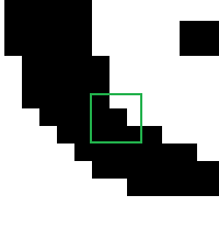
Suppose our input is a two-dimensional array corresponding to this greyscale 32 x 32 bitmap which I have blown up to examine the detail:

All of these input values are 255 (the white) or 0 (the black).

Let’s suppose our kernel is

0.0625   0.125   0.0625

0.125    0.25    0.125

0.0625   0.125   0.0625

That is, 1/16th, 1/8th, 1/16th, and so on.

Now we can compute the convolution. Remember, we’re going to do the same operation on every pixel: overlay the kernel centered on the pixel, multiply corresponding values, sum them up. Let’s suppose the current pixel we are looking at is the one in the center of the nine pixels I’ve highlighted below:

The situation is as follows:

  kernel                     overlaid on          product (rounded)

0.0625   0.125   0.0625      0   255    255       0   32    16  

0.0625   0.25    0.0625      0     0    255       0    0    16

0.0625   0.125   0.0625      0     0      0       0    0    0

The sum of the products is 64, so the old value of this pixel is the 0 in the center and the new value is 64.

Now suppose we applied that process to every pixel in the bitmap and then displayed the output bitmap as a grayscale:

We blurred it! This particular blur is called “3×3 Gaussian” and it is extremely common in graphics processing. There are many other common kernels for blurring, sharpening, edge detection, brightening, dimming, and so on. Basically the idea here is that the new value of every pixel is a weighted average of the nearby pixels; precisely how you choose those weights determines what image operation the particular convolution with that kernel performs.

That is maybe all very interesting and the next time you play some video game you can notice all the places in which graphical elements are blurred or sharpened or dimmed or whatever. But why is this relevant to Life?

Because if you take as your kernel

1  1  1
1  9  1
1  1  1

then the convolution of a Life grid with that kernel is a new grid of numbers that should seem familiar; as I mentioned at the end of episode 7, all the places in the output array that have the value 3, 10 or 11 are living cells in the next tick, and everything else is dead. The 3s are dead cells with three living neighbours, the 10s and 11s are living cells with two and three neighbours.

(Thanks once again to reader yurivkhan, whose comment on part six inspired me to add this episode; I was not initially planning on discussing image processing, but I am glad I did.)

Now, there are some issues to worry about. I completely glossed over what happened on the edges of that blur, for example. The definition of the convolution function I gave assumed that the overlaying of the kernel on the image actually overlapped, and in real graphics processing you need to specify what happens when the kernel goes “over an edge”.

What I did of course was I skipped running the convolution entirely on the edges and just kept them white. For our Life implementation, were we to use this technique, we’d probably do something similar to keep the edge permanently dead.

UPDATE: Reader Shawn Hargreaves pointed me at a sample application showing how to implement Life in C# using a convolution on a GPU, which you can find here. The kernel they are using is

2  2  2
2  1  2
2  2  2

Which, similarly, produces 5 if the cell is alive with two neighbours, 6 if dead with three neighbours, and 7 if alive with three neighbours; those cells are living in the next generation and the rest are dead. Notice also that the convolution definition specifies what edge processing algorithm to use along with the kernel. Thanks Shawn!

If we had special-purpose software libraries and hardware that could compute convolutions on large grids extremely quickly, then we could use that to get a big marginal speedup in our Life algorithms.

How big is “big”?

I am not set up to do GPU experiments on my little gaming machine here, but even cheap gaming machine GPUs can run a convolution at a rate of many hundred millions of pixels per second. Back in 2013 a graduate student did a fascinating writeup on optimizing Life on a GPU and managed to get an astonishing 20 billion cell computations per second. However, that throughput was only attained when the grid sizes became quite large, and there was considerable optimization work done to attain a fast kernel function that worked on grids that stored cells as bits.

Let’s do a quick back-of-the-envelope to see how that compares to our efforts so far.

• My best implementation so far did 5000 generations of 64k cells in 3.25 seconds, so that’s 100 million cells per second. The optimized GPU reported in 2013 is 200x faster.
• Jeroen’s SIMD did 5 million generations of 256 cells in 1 second, so that’s about 1.3 billion cells per second — though there is a bit caveat here that the program can only do 16×16 grids! A program that used SIMD instructions on larger grids would be a bit slower than 1.3 billion cells per second, but it would be in that neighbourhood. The optimized GPU is on the order of 20x faster.

I keep on coming back to this main theme: adding raw power to improve the marginal performance of an algorithm can only go so far, and we’re seeing here what the limits of that are. We are not going to do better than GPUs on any variation of the Life algorithm that works by examining every cell in a finite grid in order to determine the next tick’s grid state. GPUs are the best available technology for parallelizing simple math operations onto grids where the new cell value is a function of the near neighbours of each cell.

Moreover, an increase in speed by 200x again just means that if our previous implementation is in its performance budget for an n-quad, then throwing a GPU at the problem means that we can now do an n+3 or n+4-quad in the same time budget.

And also it is worth remembering that a GPU only has so much addressable memory on board! One expects that a typical GPU might handle something like an 8192×8192 image — a 13-quad — before it runs out of space.

We’ve found a rough upper bound on how good we can make any variation on the naive “examine every cell every time” algorithm. If we want to get better speed, we’re going to have to stop looking at every cell and counting its neighbors.

Next time on FAIC: All that said, I’m going to look at one more algorithm that examines every cell every time, but we will at least make a start at using specific characteristics of the Life problem in order to do less work. We will take an insight from this episode and see if we can use it to advantage to get a marginal advantage, and then use that as the basis for further improvements in coming episodes. Stay tuned!

Code for this episode can be found here, which — unusually — is not my GitHub repo.

Last time on FAIC I mentioned that there were two basic techniques for improving raw performance:

• keep the algorithm the same but find a marginal improvement that makes an iteration of the algorithm run faster (or use less memory, or whatever)
• find some characteristic of the problem that allows us to use a better algorithm entirely

My hope was that we’d be past the first one by now, but a number of readers and commenters have brought up points that ought to be addressed, so I’m going to spend two more episodes on the “marginal improvement” road. Specifically, on the “throw specialized hardware at the problem” technique.

I said during our discussion of Scholes’ algorithm that, though it appears to be doing exactly the same computations as the standard implementation of the naive algorithm, it is conceptually different because logically it treats the Life problem as a series of operations on matrices; that is, values. My implementation of course had a bunch of O(n) loops in it, but those loops were implementation details of the operations like “shift this matrix to the left” or “add these eight matrices together”.

What if we could actually perform matrix operations in parallel across all matrix elements at the same time? That is, truly apply the operations we’re laboriously doing byte-by-byte in each array all at once, as though they were values?

After all, we do this for the bit arrays that we call integers! When we add two 32 bit integers together we do not think of the fact that the underlying hardware is doing operations on each bit. Under what circumstances could we do the same thing to Life grids?

I’m going to discuss two techniques for this. Today, SIMD, and next time, some ideas from image processing.

It is extremely common in modern computing to wish to perform the same operation to multiple integers. Let’s say, for example, we have 44000 short (16 bit) integers representing the waveform of one second of CD audio. We’re performing some transformation on all that data in real time, as the bits are coming off the disc. Let’s say we’re reducing the volume by half. Well that’s easy enough! It’s just a one-bit unsigned shift to the right.

What would be really great though is if we could copy, say, sixteen of those short integers out of a buffer and into a 256 bit register, shift all of them to the right in parallel, and then put them back in the buffer. Plainly that would be much faster than pulling 16 bits out of the buffer, shifting it, putting it back, repeat, provided that we had hardware that could do the shifting in parallel on 16 shorts stuck into a 256 bit register.

But we do have such hardware; a great many chips now support SIMD instructions. That is Single Instruction on Multiple Data. Moreover, .NET Core provides methods that allow you to insert calls to SIMD instructions into your C# programs; if the hardware supports it, then the jitter will turn those calls into these instructions that act in parallel.

How could we use that for Life? Suppose we restricted ourselves to a 4-quad. That is, a 16 x 16 grid in my nomenclature. That’s pretty small, but we could fit a 16×16 array of cells into an array of 16 shorts if we did one bit per cell, and then we could implement Scholes’s algorithm by doing parallel bit shifts for the left and right rotations, and pointer offsets for the up and down rotations.

As it turns out, we do not have to actually suppose anything at all; we can just examine the implementation sent to me by Jeroen Frijters which does exactly that. I’m not going to go through it line by line, but I’ll hit the highlights. We can divide the program into three parts: initialization, the core stepping algorithm, and the adder. (And there is also some debug output, which I will ignore.)

Initialization is straightforward; we have a 16×16 grid and we load it into a 256 bit buffer one ushort at a time:

var v = new Vector256<ushort>()
v = v.WithElement(0x0, (ushort)0b0100_0000_0000_0000);
v = v.WithElement(0x1, (ushort)0b0010_0000_0000_0111);
...

That buffer is then dumped into an 18-ushort fixed-width array.

fixed ushort state[18];
internal Life16x16(Vector256<ushort> initialState)
{
  fixed (ushort* p = state)
  {
    Avx.Store(p + 1, initialState);
  }
}

You might not be familiar with fixed-width arrays in C#, as they are typically only ever used for unmanaged code interop scenarios and the like. The basic idea is that we allocate enough memory to hold exactly 18 ushorts, and then tell the garbage collector keep this thing still for a moment because I’m going to make a pointer into its interior. (Remember, the GC is allowed to relocate the storage associated with living objects at its discretion.)

Unfortunately this leads to some nomenclature confusion because we then have a fixed width buffer that is fixed in place and boy is it easy to get those meanings mixed up if you are not careful. I really wish the designers of C# 1.0 had used “pinned” or “immovable” or some other term to distinguish the two meanings of “fixed” in this context.

Why 18? We shall see in a moment.

That does it for the initialization phase. The heart of the algorithm is of course the step function, and let me take this opportunity to rewrite it very slightly to make it easier to understand:

fixed (ushort* p = state)
{
  var cells = Avx.LoadDquVector256(p + 1);
  var s = Avx.LoadDquVector256(p);
  var n = Avx.LoadDquVector256(p + 2);
  var e = Avx2.ShiftRightLogical(cells, 1);
  var se = Avx2.ShiftRightLogical(s, 1);
  var sw = Avx2.ShiftLeftLogical(s, 1);
  var w = Avx2.ShiftLeftLogical(cells, 1);
  var ne = Avx2.ShiftRightLogical(n, 1);
  var nw = Avx2.ShiftLeftLogical(n, 1);

We copied the 16 ushorts worth of board state into the interior of the 18 byte buffer, so that there would be an all-zero word at the top and bottom. That way the “shift north” and “shift south” operations are nothing more than reading the bits starting from the first and third ushorts in the fixed-size array.

The shifts to the east and west are done in parallel on all 256 bits in the vector. Something to keep in mind here is that this is not a right or left shift of a 256 bit integer! That would be wrong because the edges would wrap incorrectly. Rather, it is truly doing a single shift-by-one operation on each of the 16 ushorts in the bit vector, so we get a zero bit on the left or right appropriately. Recall that when I implemented this a couple episodes ago on a byte array I needed to add code to ensure that zeros were filled in appropriately, but here we get that for free from the hardware.

We then have the remainder of Scholes’ algorithm, though it is slightly more verbose than I wrote:

var acc = new FourBitAccumulator(se, s, sw, e);
acc.Add(cells);
acc.Add(w);
acc.Add(se);
acc.Add(n);
acc.Add(sw);
Avx.Store(p + 1, Avx2.Or(acc.IsThree, Avx2.And(acc.IsFour, cells)));

What’s happening here is we have a helper class that implements the “add these nine bit vectors together to get the living neighbor count”, which of course fits into four bits.

We then do the same thing as before: call helper methods to find all the threes and living fours, and that’s our next generation.

The remainder of the program is a four-bit parallel adder that also uses SIMD instructions to add all nine 256 bit vectors together in parallel, which produces four 256 bit vectors each of which has one bit of the sum. Going through the code to verify that it is a correct adder is tedious and spoiler alert, it is correct, so I’ll skip that.

What kind of performance boost would we get if we used this thing? We can do a quick calculation to get an order of magnitude.

My implementation of Scholes’ algorithm took 3.25 seconds to compute 5000 generations of an 8-quad — that is, a 256×256 cell grid. That works out to 100 megacells/s.

I did a quick performance check of this algorithm and I got 5 million ticks per second, but only doing the work on 256 cells. That’s 1.3 gigacells/s, 13 times faster on a cells-per-second basis. That seems like the right order of magnitude speedup considering that all the work is being done in parallel.

Now, of course scaling this algorithm up to use SIMD instructions on 8-quads would not be simply doing 256 times the work as was done on a 4-quad because we cannot use the fact that the north, south, east and west shifts put zeros along the edges! We need those bits to be filled in with the correct bits from the grid state, and that’s going to be many additional instructions, so maybe this would only be 10x or 8x faster after that. But 8x faster is pretty good.

On the other hand, remember what our scalability problem is here. Every time we double the width of the grid we get 4x as many cells in it. So what this means is that if an n-quad is within our performance budget for my unoptimized algorithm, then an (n+1) or maybe if we are lucky, an (n+2) quad is in our budget for this SIMD version assuming we could scale it up to larger grids. It doesn’t sound like nearly so great an increase when you look at it that way.

Many thanks to Jeroen for inspiring this episode and providing the code. Next time on FAIC we’ll finish off our discussion of parallelism with a quick introduction to a basic image processing technique that is germane to our topic.

Last time on FAIC we took a look at Scholes’ extremely concise Life algorithm, which treats a grid as an array that you can treat as a mathematical value with some unusual but entirely straightforward manipulations. We didn’t get the same concision in C# as you would in APL, but I’m OK with that.

I won’t go through the same level of detail discussing the asymptotic performance of this algorithm as I did for the naïve algorithm. If we have n cells in the array then we do eight array manipulations, each of which allocates an array of size n and fills it in; each of these operations will be O(n). Similarly, the “Where” and “or” operations are O(n), and so the whole thing is O(n).

This shouldn’t be a surprise; this is in many ways just the naïve algorithm again! We do almost exactly the same work — we compute the sum of the living neighbors of every single cell, and set the new cell state based on that sum and each cell’s current state. We just do the operations in a slightly different order.

What about actual time and memory performance?

Plainly this algorithm as I have implemented it takes more temporary memory; it allocates thirteen arrays as it goes, and those arrays are then garbage that needs to be collected. The optimized version of the naive algorithm allocates only two arrays and it keeps both of them alive, so neither becomes garbage.

The garbage is at least short-lived and so will be collected quickly. But in my example of an 8-quad (256×256) byte array, we get in under the limit for allocation on the Large Object Heap. Things might be different if we moved up to a 9-quad because then all these temporary arrays would be large objects, and the GC assumes that large objects live longer. I haven’t tried it out to see what the impact is.

What about time?

As I said in a previous episode, when I make a performance prediction I am on average dead wrong maybe a third of the time. We saw that on my machine, after some small amount of very straightforward performance tuning the naïve algorithm took about 4 seconds to do 5000 ticks of an 8-quad; my prediction was that since Scholes’ algorithm is doing all the same amount of work, and allocating 13 temporary arrays as it goes, that it would be around the same but slightly slower due to all the copying.

Imagine my astonishment then when I discovered that my implementation of Scholes algorithm without any perf work at all took 3.25 seconds to do the same problem. Nearly 20% faster! I must confess, I do not know what is going on here, but I do know that those array copy steps are extremely fast. Unfortunately I do not have the time right now do to a detailed perf analysis to figure out what is going on here; if anyone has insights, please leave a comment.

Let me finish up this episode with three additional thoughts:

First, I noted last time that the algorithm I implemented is inspired by Scholes’ APL algorithm but is not exactly the same. How is it different?

The big thing is that my “array shift” operations are different than the array “rotations” used in the APL algorithm. That is, my “shift left” would transform an array like this:

1 2 3                      2 3 0
4 5 6  --shift left->      5 6 0
7 8 9                      8 9 0

Whereas I believe — any APL aficionados reading this please confirm or deny — that the APL rotation is:

1 2 3                      2 3 1
4 5 6  --rotate left->     5 6 4
7 8 9                      8 9 7

And similarly for shifting right, up and down.

I mentioned several episodes back that a standard technique for implementing Life algorithms is to make the edges of a finite grid “wrap around”, effectively making the board a torus. That’s what this algorithm does if you use this array rotation, and if you watch the video I linked in the previous episode you will see that in fact the given code implements wrap-around Life.

Second, I implemented the byte block data type in the least sophisticated manner possible: allocate an array on every operation. There are other ways to store data to make the sorts of operations we’re doing involve fewer array copies, and those could possibly reduce the time and memory consumption further. If you are clever (and the arrays are immutable) then you can instead of making a copy, instead just keep the original array and do a little extra math on every array read.

Though it would be interesting to know how much of an improvement (or regression!) those kinds of optimizations would achieve, I don’t want to spend too much time digging into this one algorithm. If anyone wants to do the experiment, please do and report back.

Third, one of the themes of this series that is emerging is that there are two basic ways to attack a performance problem:

• Keep the algorithm basically the same but find a marginally faster way to implement it. For instance: avoid array bounds checks by using unsafe pointer arithmetic, or throw specialized libraries or hardware at the problem. This does not improve asymptotic performance or scalability but it can lead to small or large wins in raw performance on problems of a specific size.
• Find some characteristic of the specific problem under investigation that enables us to come up with a new algorithm that does less work or uses less space or has less GC burden. This often gives us an improvement in asymptotic performance, and therefore changes how we can scale up to larger problems.

So far we’ve been concentrating entirely on the first family of techniques; we will get to the second soon!

I intended in this episode to talk a bit about the “use specialized hardware to attack the problem” technique, but I think this episode is long enough for today, so let’s pick up there next time.

Next time on FAIC:  I’ll present an implementation submitted by a reader that uses specialized hardware instructions to implement Scholes’ algorithm on a 4-quad.

Code for today’s episode can be found here. I’ve added drag scrolling to the user interface, so if you click and hold, you can move around the grid much the same way that you’d move around an online map site.

Thanks to Java language designer Brian Goetz for being the first to suggest this episode’s topic. A number of other commenters here and on Twitter have suggested this and similar techniques; I will present a slightly simplified C# implementation of the algorithm today, and then next time I’ll discuss the performance implications, including those of using specialized hardware.

For the last few episodes we’ve been digging into the naïve algorithm: make an array of bools — or, in our rewrite, bytes — examine each neighbor of each cell, and fill in the new array accordingly. We’ve done some basic performance optimizations and managed to get it to about 1250 steps per second on an 8-quad, which seems pretty good.

Today I’m going to take a look at an approach that is similar in effect — we’re still going to have a byte array the size of the grid, and we’re still going to count the neighbors of each cell, but the order in which we do the operations and how we carry them out is going to be completely different.

The algorithm that I’m going to present here was developed by noted APL programmer, the late John Scholes. The original implementation of this algorithm is a single line:

life ← {⊃1 ⍵ ∨.∧ 3 4 = +/ +⌿ ¯1 0 1 ∘.⊖ ¯1 0 1 ⌽¨ ⊂⍵}

APL is a famously difficult language to understand because it is written in its own extraordinarily terse notation. I am not going to attempt to unpack this implementation! If you want an explanation, you can watch John Scholes explain it himself in this video:

Or, what I found more clear, is to follow along slowly in this article.

Rather than try to explain how this works in APL, I’m simply going to develop an algorithm that is in spirit pretty much the same as the one Scholes presents. It will differ in the implementation details — I’ll discuss how in the next episode — and will certainly be easier to read for the non-APL programmer. But the basic idea will be the same.

The key to understanding what is going on here is to first take a step back and understand what APL is for in the first place. It is a language for expressing algorithms that operate on multidimensional arrays. Since we’ve seen that we can implement a subset of the infinite Life grid in a 2-d array of bytes, each of which is 0 or 1, it seems plausible that a language specifically designed for array operations should be able to handle Life no problem.

APL can of course handle arbitrarily complex tensors, but we won’t need that machinery for the purposes of this discussion; all we need is a 2-d array of bytes. Thus I’m going to start by making my own “2-d array of bytes” type; it will be a class that is just a thin wrapper around a 1-d byte array. (We’ll see why I prefer the underlying implementation to be a 1-d byte array in a minute.)

class ByteBlock
{
  private int Width { get; }
  private int Height { get; }
  private readonly byte[] bytes;
  public ByteBlock(int width, int height, byte[] bytes = null)
  {
    this.Width = width;
    this.Height = height;
    this.bytes = bytes == null ? new byte[width * height] : bytes;
  }

Obviously I’ve omitted error detection and whatnot for the purposes of keeping it short on the blog.

For the majority of the operations I’m going to perform on this type, byte blocks will be immutable. However it is convenient to be able to edit one without creating a bunch of garbage blocks, so I’ve added a getter and a setter; I’ll omit the details as they are very obvious. See the source code if you’re interested.

So far there is nothing out of the ordinary, but now let’s make it slightly more interesting. I want to add eight operations to this type, starting with “move left”:

1 2 3                   2 3 0
4 5 6  ---move left-->  5 6 0
7 8 9                   8 9 0

That is: “move left” produces a new byte block with the same size, but all the entries shifted one space left. The space left behind is filled in with zeros. (Again, this is slightly different from the APL vector rotation operation described by Scholes, and I’ll discuss why that is in an upcoming episode. I don’t want this first explanation to be overwhelmed by digging into subtleties.)

How can we implement that?  Well, we have a one-dimensional array underlying this thing, so let’s just copy everything one unit to the left, and then fill in the zeros where we need to!

public ByteBlock MoveLeft()
{
  byte[] newBytes = new byte[bytes.Length];
  Array.Copy(bytes, 1, newBytes, 0, bytes.Length - 1);
  for (int i = Width - 1; i < newBytes.Length; i += Width)
    newBytes[i] = 0;
  return new ByteBlock(Width, Height, newBytes);
}

Easy peasy. Now do exactly the same for MoveRight, MoveUp and MoveDown; the code is straightforward and so I’ll skip posting it here.

APL of course has a fully featured library of these sorts of array transformations, being an array language, but I just need four more.

“Where” takes a value and produces a new block which is one everywhere the original block has that value and zero everywhere else:

1 2 3                   0 0 0
4 5 6  ---where 4-->    1 0 0
7 8 9                   0 0 0

public ByteBlock Where(byte b)
{
  byte[] newBytes = new byte[bytes.Length];
  for (int i = 0; i < bytes.Length; i += 1)
    newBytes[i] = bytes[i] == b ? (byte)1 : (byte)0;
  return new ByteBlock(Width, Height, newBytes);
}

I need “and” and “or” operators that take two byte arrays of the same size and do the appropriate operation on each corresponding element of each array. And I need a “sum” operator that takes any number of byte arrays of the same size and produces the array that is the sum of each element.

I’ll make Sum an instance method that takes a param array of additional summands, and make the bitwise operators via operator overloading. You see how this goes; I don’t need to spell it all out; see the code on GitHub if you care about the details.

Once we have these tools, what do we do?

A Life grid is exactly the same as it was in the optimized naïve implementation: a 2-d array of bytes where each byte is 1 if the cell is alive and 0 if it is off, but this time we’re going to represent the cells as a byte block:

class Scholes : ILife
{
  private const int height = 256;
  private const int width = 256;
  private ByteBlock cells;
  public Scholes()
  {
    Clear();
  }
  public void Clear()
  {
    cells = new ByteBlock(width, height);
  }

Pretty straightforward. I’ll skip the boilerplate getter/setter code and get straight to the crux of the matter: how does Next work?

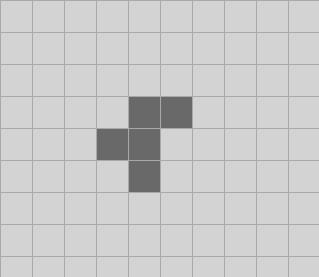
The article I linked to above does a great job of explaining by running a simple example, so I’m going to do exactly the same thing; don’t mess with success. The R-pentomino is the smallest original configuration that runs for a long time before it gets to a stable configuration of still lifes, oscillators and gliders. The initial state is:

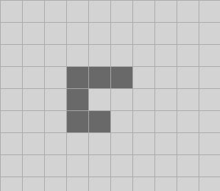
And one tick later:

It then takes 1103 ticks to settle down, but we’ll just worry about the first two. This is a good example because it has almost every case in it: we have living cells with 2 and 3 living neighbors that survive, we have living cells that die from overcrowding, and we have dead cells that stay dead and dead cells that come alive. (Though as we will see in a moment, there is a slightly different reason why this is a good test case!)

I’ll just focus on the 5×5 subset of the grid centered on the pentomino, and for compactness I’ll remove all the spacing between the grid values; none will ever go over nine. So we start with:

cells:
00000
00110
01100
00100
00000

You know what? That’s hard to read. I’m going to replace the zeros with dots, as in the video I linked above:

cells:
.....
..11.
.11..
..1..
.....

The first thing we do is move it up, down, left and right, or, if we think of this as if we were reading a standard map, we moved them west, east, north and south:

var w = cells.MoveLeft();
var e = cells.MoveRight();
var n = cells.MoveUp();
var s = cells.MoveDown();

  w     e      n      s
.....  .....  ..11.  .....
.11..  ...11  .11..  .....
11...  ..11.  ..1..  ..11.
.1...  ...1.  .....  .11..
.....  .....  .....  ..1..

Next thing we do is do an additional two moves on the “east” and “west” blocks; effectively these have moved the original pattern to the northwest, northeast, southwest and southeast if we think of it as a map.

var nw = w.MoveUp();
var ne = e.MoveUp();
var sw = w.MoveDown();
var se = e.MoveDown();

  nw    ne     sw     se
.11..  ...11  .....  .....
11...  ..11.  .....  .....
.1...  ...1.  .11..  ...11  
.....  .....  11...  ..11.
.....  .....  .1...  ...1.

Now sum all of those eight new block with the original block.

var sum = cells.Sum(w, e, n, s, nw, ne, sw, se);

01221
13431
14541
13320
01110

All right, what have we got? We have an array where every entry in it is equal to the original value plus the count of all the living neighbors! The sum in the very middle, 5, for instance, is 1, the original value of the cell, plus the number of living neighbors, 4.

Now that we have this information, what can we do with it? We observe:

• If a cell was alive and it had two living neighbors, the sum is 3, and it will be alive on the next tick.
• If a cell was alive and it had three living neighbors, the sum is 4, and it will be alive on the next tick.
• If a cell was dead and it had three living neighbors, the sum is 3, and it will be alive on the next tick.
• Everything else is dead on the next tick.

(And now we see why I said before that this was a good test case; we have sums of both three and four on cells that were alive and dead previously.)

We have everything we need to make it happen. All the cells where sum is 3 are alive:

var threes = sum.Where(3);

.....
.1.1.
.....
.11..
.....

All the cells where the sum is 4 and the original cell was alive are alive:

var fours = sum.Where(4);
var livingFours = fours & cells;

.....
..1..
.1...
.....
.....

Finally…

cells = threes | livingFours;

.....
.111.
.1...
.11..
.....

And we’re done!

(Technically I guess we didn’t really need “or” because the threes and living fours arrays are necessarily disjoint; we could have just summed them. But I think conceptually it makes good sense to think of this as an “or” rather than a sum.)

Let’s put it all together; it’s not nearly as concise as APL because nothing is, but it is pretty short:

public void Step()
{
  var w = cells.MoveLeft();
  var e = cells.MoveRight();
  var n = cells.MoveUp();
  var s = cells.MoveDown();
  var nw = w.MoveUp();
  var ne = e.MoveUp();
  var sw = w.MoveDown();
  var se = e.MoveDown();
  var sum = cells.Sum(w, e, n, s, nw, ne, sw, se);
  cells = sum.Where(3) | sum.Where(4) & cells;
}

I find it really quite pleasant to read the algorithm like this.

There are numerous other ways to use this same sort of technique to get what we want, of course; user yurivkhan pointed out in a comment to episode six that if we add a “multiply by scalar” operation that multiplies each value in a byte array by the same value, then this is the same computation just expressed a different way:

 var sum = (cells * 8).Sum(w, e, n, s, nw, ne, sw, se);
 cells = sum.Where(3) | sum.Where(10) | sum.Where(11);

( I’ll address yurivkhan’s further comments about image processing techniques in the next episode.)

Next time on FAIC: We’ll look at the asymptotic, memory and time performance of this algorithm and its implementation, and discuss how ideas from image processing can improve the raw speed.

Code for this episode can be found here. The only interesting change I’ve made to the client is that if you press “P”, it pauses the simulation and runs 5000 steps of the “acorn” pattern, and then dumps the number of milliseconds that took to a text file. This is a quick and dirty performance test, but as we’ll see, we can get great results even with this primitive tool.

Last time we demonstrated that a single tick in the naïve “array of bools” algorithm is O(n) in the number of cells, which is not surprising — after all, we do a neighbor count of every cell on every tick. This gives us the insight that if we quadrupled the number of cells, we’d probably quadruple the time to compute a step, which is good to know, but we still don’t know how bad it is, aside from noting that we’re having no problem keeping up with a cadence of two ticks per second of course!

As I mentioned in the preamble, I wrote the quickest little perf tester you could imagine and ran it on the release version of the app. There is no point in running performance testing on a debug app, or on a release app while it is running in the debugger; remember, the runtime knows it is being debugged and changes the performance characteristics of the program in order to make it easier to debug.

On my home machine — a decidedly mediocre mid-end PC game box — I got 5000 steps of “acorn” in 17 seconds, which is around 300 steps per second. By 1992 standards, that would be insanely great, but let me tell you, machines are a lot faster today than they were in 1992.

I did not deliberately “sandbag” this implementation — I did not write it to have a deliberately slow bit — so there’s no trick to figuring out where we’re spending time. I wrote it with an emphasis on clarity and correctness, knowing that we could come back later and find the hot spots; it’s a lot easier to optimize code if it is already clear and correct.

The question now is: where would you guess most of the time is being spent in the calculation? (Remember, we are omitting the time to draw to the bitmap.)

If you didn’t have a profiler on your machine — and I don’t! I have the free version of VS on my home machine — what would your gut tell you? Because my gut is almost always at least partially wrong when it comes to performance.

Let’s quickly review the naïve algorithm. The major parts are:

Test to see if a point is inside our 8-quad of valid cells:

private bool IsValidPoint(long x, long y) => 
  0 <= x && x < width && 0 <= y && y < height;

Fetch the value from the array if the point is valid; dead otherwise:

public bool this[long x, long y]
{
  get
  {
    if (IsValidPoint(x, y))
      return cells[x, y];
    return false;
  }

Count the neighbors:

private int LivingNeighbors(int x, int y)
{
  int sum = this[x - 1, y - 1] ? 1 : 0;
  sum += this[x - 1, y] ? 1 : 0;
  sum += this[x - 1, y + 1] ? 1 : 0;
  sum += this[x, y - 1] ? 1 : 0;
  sum += this[x, y + 1] ? 1 : 0;
  sum += this[x + 1, y - 1] ? 1 : 0;
  sum += this[x + 1, y] ? 1 : 0;
  sum += this[x + 1, y + 1] ? 1 : 0;
  return sum;
}

And the main loop:

bool[,] newCells = new bool[width, height];
for (int y = 0; y < height; y += 1)
  for (int x = 0; x < width; x += 1)
  {
    int count = LivingNeighbors(x, y);
    newCells[x, y] = count == 3 || (cells[x, y] && count == 2);
  }
cells = newCells;

So, no peeking below: without a profiler to guide you, what would you assume was the low-hanging fruit that could be attacked here to make the whole thing a little faster without changing the basic algorithm or data structures?

I find that I’m dead wrong about a third of the time when I look at a piece of code and guess where the time is being spent, and fortunately this was one of the times I guessed correctly. The biggest cost by far in this loop is that it calls IsValidPoint eight times on every loop iteration. Since there are 65536 loop iterations per tick, that’s over two billion validity checks in our performance run.

Moreover, the vast majority of the time, the point is valid; the only “invalid” points we generate are when looking for neighbors when on edges.

How can we improve this? The easiest way is just to note that we have two cases, the interior points where all neighbors are valid, and the edges where not all neighbors are valid. If we are in the former case, which we can check for once, then we can skip all the other validity checks:

if (1 <= x && x < width - 1 && 1 <= y && y < height - 1)
{
  int sum = cells[x - 1, y - 1] ? 1 : 0;
  sum += cells[x - 1, y] ? 1 : 0;
  ...
  return sum;
}
else
{
  // as before:
  int sum = this[x - 1, y - 1] ? 1 : 0;
  ...

Making this change takes us from 5000 ticks in 17 seconds to 4.4 seconds.That’s a 4x improvement right there!

That was no surprise at all, but my experiments with making further tweaks to the code were quite surprising. Before I get into the details, let me hasten to say: I have not actually looked at the generated assembly to figure out why the jitted code has non-obvious performance characteristics, but I have some educated guesses. Take everything below with a grain of salt, and if anyone cares to look at the generated machine code to confirm or deny my guesses, I’d be happy to make an update.

Here are some things I tried to see if they made an improvement or a regression; I’ll list the winners first:

I wondered if we were paying any penalty for all these conditionals:

int sum = cells[x - 1, y - 1] ? 1 : 0;

On the one hand, the Boolean should be represented as a byte that is either zero or one, so the jitter could make the conditional a no-op, right?

On the other hand, there are sneaky ways to make a Boolean contain a non-zero, non-one value, and those should all be treated as true, but that would make the “turn this conditional into a no-op” optimization invalid.

Like I said above, I haven’t checked the codegen to see what exactly it does. But when I turned the bool array into a byte array and removed the conditionals, that trimmed an additional 40 microseconds off of each step for a total of 200 milliseconds over 5000 steps.

Allocating a lot of new arrays has two costs: it has to initialize the new array to zero, and it causes collection pressure which increases the number of GCs. (Fortunately we are sneaking in under the 85K limit for arrays to avoid going on the Large Object Heap, but we’re very close, and that would change things as well.)

This algorithm fills in every element in the new array, so there’s no need for it to be initialized at all, or allocated and then immediately freed.

If we go to a solution where we cache the temporary array and re-use it, that shaves off another 200 milliseconds over 5000 steps.

When I was working on the nullable lowering code in the compiler I learned that if we were generating, say, an addition of two nullable integer values x and y, that you always generate the code as if the user wrote:

result = x.HasValue() & y.HasValue() ? ...

and not

result = x.HasValue() && y.HasValue() ? ...

Why’s that? Because checking whether x has a value and branching if it does not is more expensive than simply calling y.HasValue()! Avoiding the work is more expensive than just doing it. And moreover, every branch is a new basic block, and basic blocks make the jitter work harder and therefore potentially skip more optimizations; the jitter has to be fast.

I therefore wondered if I could rewrite

  if (1 <= x && x < width - 1 && 1 <= y && y < height - 1)

which after all is just

  if (1 <= x)
    if (x < width - 1)
      if (1 <= y)
        if (y < height - 1)

as instead

  if (1 <= x & x < width - 1 & 1 <= y & y < height - 1)

Turns out, that’s actually a small regression. This was suprising, particularly since the conditions are almost always true and therefore you don’t get much savings by avoiding work on the edges.

I’m not sure what’s going on here, but I have a guess. Let’s look at the other losers and then I’ll theorize further at the end.

As we’ve seen, the special-purpose code for handling the edges is a source of pain because we do extra work to not dereference outside the array. A standard technique for Life on finite grids is to make a “rectangle of death” along the edge. That is, allocate memory for a 256×256 grid, but only actually do the computations on the 254×254 grid on the interior, and keep the 1000 or so cells on the edges permanently dead. We waste a couple KB of memory, but we save time on not having to constantly check whether we’re computing neighbors of an edge cell because we just skip them entirely.

When I only restricted the computations to the interior by changing the loop conditions, of course we were now doing 1000 fewer cells than before, so there was a commensurate speedup. But here’s the weird bit. When I removed the now unnecessary:

if (1 <= x && x < width - 1 && 1 <= y && y < height - 1)

check, the program got slightly but consistently slower.

What the heck? It’s doing less work, so how did it get slower?

This code seems to be doing some recomputation:

int sum = this[x - 1, y - 1] ? 1 : 0;   
sum += this[x - 1, y] ? 1 : 0;
...

We recompute x-1, x+1, y-1 and y+1 several times.

When I put those into local variables to avoid recomputing them, again I got a small but consistent regression!

Finally, the one that was most surprising to me. It is fairly well-known that in .NET, the jitter does a better job optimizing operations on single-dimensional arrays than multi-dimensional arrays. I tried changing my cell array to a single-dimensional array, and then accessed it as

cells[x + y * width]

throughout. This also caused a small regression!

I have a hypothesis that explains these unexpected regressions.

Arrays are memory-safe in C#. Accessing a single-dimensional array outside its bounds throws an exception, and accessing a multi-dimensional array outside of any of its bounds is an exception even if the offset computed into the underlying memory block would be in range.

The jitter has a lot of smarts in it to avoid doing unnecessary bounds checks. In particular, if you have:

for(i = 0; i < a.Length; a += 1)
  sum += a[i]

Then the runtime knows that the array access inside the loop will always be in bounds, so it skips emitting a bounds check.

I suspect that what is going on here with all of these unexpected regressions is that the edit causes the jitter to fall out of a “known to be good” path and it starts generating more array bounds checks.

We are smart enough to know that the array indices will be in bounds, but the jitter only has a very small time budget to analyze a method body; as I noted above, it makes no sense to do a work-avoiding optimization if determining whether the optimization applies costs more than the work saved!

This is just a conjecture though; if anyone knows for sure what is going on here, I’d love to see a deeper analysis.

The obvious comment here is “can we avoid the checks entirely by going to unsafe code?” I’ll address that point in a later episode, so hold off there for now!

Summing up:

• Our tweaked algorithm, which you can find in BoolArrayOpt.cs, goes from 17 seconds to 4 seconds for 5000 ticks, or 1250 ticks per second. That seems decent for an early attempt.
• If we get 1250 TPS with an 8-quad, then we should get about 80 TPS with a 10-quad and about 20 with an 11-quad, so a 1024×1024 grid is about as good as we can get with this implementation if we want to meet our performance goal of animating smoothly. I have not actually tried it though; it would be interesting to see what the scaling factor really is.
• The moral of the story here is performance of managed code can be surprising, so always measure! 

Next time on FAIC: there’s a (seemingly) completely different flavor of array-based solution to this problem that I’d like to spend an episode or two digging into.