Here we go again!

Fellow BASIC enthusiast Jeff “Coding Horror” Atwood, of Stack Overflow and Discourse fame, has started a project to translate the programs in the 1978 classic BASIC Computer Games into more modern languages. I never had a copy of this one — my first computer book was Practise Your BASIC — but these programs are characteristic of the period and I am happy to help out.

1978 was of course well into the craze of writing Life simulators for home personal computers. In this episode I’ll break down the original program assuming that you’re not a BASIC old-timer like me; this language has a lot of quirks. You can read the commentary from the book here, and f you want to run the original program yourself the copy here is a valid Vintage BASIC program.

Let’s get into it!

2 PRINT TAB(34);"LIFE"
4 PRINT TAB(15);"CREATIVE COMPUTING  MORRISTOWN, NEW JERSEY"
6 PRINT: PRINT: PRINT
8 PRINT "ENTER YOUR PATTERN:"

• All lines are numbered whether they need to be or not. Line numbering is often used to indicate program structure; we’ll come back to this in a bit.
• Lines are not one-to-one with statements! A single line may contain several statements separated by colons.
• PRINT takes a semicolon-separated list of zero or more expressions.
• PRINT outputs a newline by default; as we’ll see presently, there is a way to suppress the newline.
• TAB(x) does not produce a string; it moves the “print cursor” to column x. In many versions of BASIC, TAB can only appear as an argument to PRINT.

9 X1=1: Y1=1: X2=24: Y2=70
10 DIM A(24,70),B$(24)
20 C=1

• Variable names are typically one or two characters.
• 24 x 70 is the size of the Life board that we’re simulating here; this was quite a large screen by 1978 standards. I owned both a Commodore 64 and a Commodore PET with 40×25 character screens; it was possible to get an 80-column PET but they were rare.
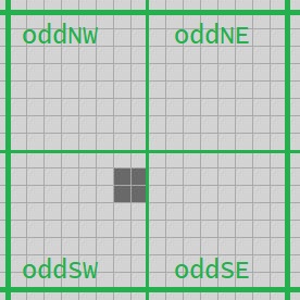
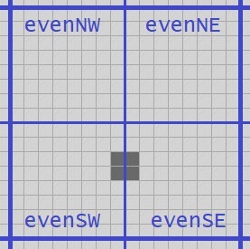
• Note that the authors have made the bizarre choice throughout that (X, Y) coordinates refer to (line, column) and not the more standard (column, line) interpretation. Normally we think of X as being the left-right coordinate, not the top-bottom coordinate.
• Single-valued variables need not be declared.
• Array-valued variables are “dimensioned”, and the dimensions typically must be literal constants. Here we have a two-dimensional array and a one-dimensional array.
• Anything that is string-valued has a $ suffix, so B$ is an array of strings.
• Arrays and strings are both indexed starting from 1.
• As we know from early episodes in this series, a naïve implementation needs to keep track of both the “current” and “next” state. In a memory-constrained environment such as can be assumed by a 1978 BASIC program’s author, we need to keep all that in the same array. Spoiler alert: the convention used by this program for the contents of array A is:
  • 0 means cell is dead, will stay dead.
  • 1 means cell is alive, will stay alive.
  • 2 means cell is alive, will die.
  • 3 means cell is dead, will come alive.
• You might have noticed that the program is formatted to have very few unnecessary spaces. Having become accustomed to vertical and horizontal whitespace being used to reduce eyestrain and guide the reader, it looks dense and hard to read. This was not a stylistic choice though; it was imposed by the limitations of the technology of the time. Line lengths were constrained, often to the width of the screen, and when you have only 40 or 80 characters of screen, unnecessary spaces are bad. But more interesting from my perspective as a compiler writer is that implementations of BASIC often tokenized as the user typed in the program, and then stored only the tokens in memory, not the original source code as it was typed. When the program was listed back, the program printer reconstituted the program from the token stream which had discarded the spaces. Pre .NET versions of VB did this!

30 INPUT B$(C)
40 IF B$(C)="DONE" THEN B$(C)="": GOTO 80
50 IF LEFT$(B$(C),1)="." THEN B$(C)=" "+RIGHT$(B$(C),LEN(B$(C))-1)
60 C=C+1
70 GOTO 30

• INPUT takes a string from the console and places it in the given variable.
• Arrays are indexed using parentheses.
• This is a “while” loop but most BASICs did not have loop structures beyond FOR/NEXT, or even ELSE clauses for IF/THEN statements. You had to write GOTO statements to build those control flows, as shown here. Notice that all the colon-separated statements execute if the condition of the IF is met; otherwise we continue on to the next statement. (I was fortunate to have access to an original PET with Waterloo Structured BASIC which did have while loops, though I did not understand the point of them when I was in elementary school. Many years later I ended up working with some of the authors of Waterloo BASIC in my first internships at WATCOM, though I did not realize it at the time! The whole saga of Waterloo Structured BASIC and the SuperPET hardware is told here.)
• LEFT$, RIGHT$ and LEN do what they say on the tin: give you the left substring of given length, right substring of given length, and length of a string. Strings are not directly indexable.
• + is both the string concatenation operator and the arithmetic addition operator.
• It seems clear that we are inputting strings and sticking them in an array until the user types DONE, but why are we checking whether the first character in the string is a period, and replacing it with a space? It is because in some versions of BASIC, INPUT strips leading spaces, but they are necessary when entering a Life pattern.
• Did you notice that nothing whatsoever was explained to the user of the program except “enter your pattern”? Enter it how? Why should the user know that spaces are dead, leading spaces are soft, a period in the first place is a hard space but a live cell anywhere else, and that you type DONE when you’re done? The assumption of the authors is that the only person running the code is the person who typed it in. “You should explain as little as possible” is not a great attitude to drill into beginner programmers.
• Notice that we have no bounds checking. B$ was dimensioned to 24 elements; if the user types in more than 24 lines in the pattern, the program crashes. Similarly we have no checks on the lengths of the strings themselves. A whole generation of young programmers was taught from their very first lesson that crashes are the user’s fault for doing something wrong.
• Our program state by the time we break out of the loop is: B$ has C lines in it, and B$(C) is an empty string.

80 C=C-1: L=0
90 FOR X=1 TO C-1
100 IF LEN(B$(X))>L THEN L=LEN(B$(X))
110 NEXT X

• Since the last line is always blank, we are reducing the line count C by one.
• The maximum line length L is initialized to zero, unnecessarily. I prefer an unnecessary but clear initialization to the lack thereof. But as we’ll see in a moment, some variables are just assumed to be initialized to zero, and some are initialized twice needlessly. More generally, programs that were designed to teach children about programming were chock full of sloppy inconsistencies and this is no exception.
• FOR/NEXT is the only structured loop in many early BASICs. The loop variable starts at the given value and executes the body unless the loop variable is greater than the final value. Some versions of the language also had an optional STEP clause, and some would even keep track of whether the loop was counting up or down. Fancy!
• Plainly the purpose of the FOR/NEXT loop here is to find the maximum line length of the pattern input by the user, but it appears to have a bug; we have strings in B$ indexed from 1 through C, but we are skipping the length check on B$(C). The subtraction here appears to be a mis-edit; perhaps the C=C-1 was moved up, but the developer forgot to adjust the loop condition. The bug only affects inputs where the last line is also the longest.
• Is it inefficient to compute LEN(B$(X)) twice in the case where the maximum length L needs to be updated? Many versions of BASIC used length-prefixed strings (as do all versions of VB and all .NET languages) and thus computing length is O(1). When I first learned C as a teenager it struck me as exceedingly weird that there was no out-of-the-box system for length-prefixing a string. And it still does.

120 X1=11-C/2
130 Y1=33-L/2
140 FOR X=1 TO C
150 FOR Y=1 TO LEN(B$(X))
160 IF MID$(B$(X),Y,1)<>" " THEN A(X1+X,Y1+Y)=1:P=P+1
170 NEXT Y
180 NEXT X

• There are no comments in this program; it would be nice to explain that what we’re doing here is trying to center the pattern that the user has just typed in to the interior of a 24 x 70 rectangle. (X1, Y1) is the array coordinate of the top left corner of the pattern as it is being copied from B$ to A; spaces are kept as zero, and non-spaces become 1. This automatic centering is a really nice feature of this program.
• Once again we have no bounds checking. If L is greater than 67 or C is greater than 23, bad things are going to happen when we index into A. (Though if C is greater than 23, we might have already crashed when filling in B$.)
• We already initialized X1 and Y1; we have not read their values at any point before they are written for a second time. By contrast, the population count P is accessed for the first time here and is assumed to be initialized to zero. Again, there is some amount of sloppiness going on here that could have been easily removed in code review.

200 PRINT:PRINT:PRINT
210 PRINT "GENERATION:";G,"POPULATION:";P;: IF I9 THEN PRINT "INVALID!";
215 X3=24:Y3=70:X4=1: Y4=1: P=0
220 G=G+1
225 FOR X=1 TO X1-1: PRINT: NEXT X

• The input and state initialization phase is done. This is the start of the main display-and-compute-next-generation loop of our Life algorithm. The subtle indication is that the line numbering just skipped from 180 directly to 200, indicating that we’re starting a new section of the program.
• Notice that two of our PRINT statements here end in semicolons. This suppresses the newline at the end. Notice also that the separator between G and “POPULATION:” is a comma, which instructs PRINT to tab out some whitespace after converting G to a string and printing it.
• I9, whatever it is, has not been initialized yet and we are depending on it being zero. There is no Boolean type; in BASIC we typically use zero for false and -1 for true. (Do you see why -1 for true is arguably preferable to 1?)
• We know that (X1, Y1) is the top left corner of the “might be living” portion of the pattern inside array A. (X2, Y2) and (X3, Y3) both appear to be the bottom right corner of the array, both being (24, 70) at this point, and (X4, Y4) is (1, 1), so it is likely another “top left” coordinate of some sort. Maybe? Let’s see what happens.
• We reset the living population counter P to zero and increase the generation count G by one.
• We then print out X1-1 blank lines. This implementation is quite smart for a short 1978 BASIC program! It is tracking what subset of the 24×70 grid is “maybe alive” so that it does not have to consider the entire space on each generation.
• We’re continuing with the pattern established so far that X and Y are loop variables. Thankfully, this pattern is consistent throughout the program.
• The assignment of P on line 215 is redundant; we’re going to assign it zero again on line 309 and there is no control flow on which it is read between those two lines.

230 FOR X=X1 TO X2
240 PRINT
250 FOR Y=Y1 TO Y2
253 IF A(X,Y)=2 THEN A(X,Y)=0:GOTO 270
256 IF A(X,Y)=3 THEN A(X,Y)=1:GOTO 261
260 IF A(X,Y)<>1 THEN 270
261 PRINT TAB(Y);"*";
262 IF X<X3 THEN X3=X
264 IF X>X4 THEN X4=X
266 IF Y<Y3 THEN Y3=Y
268 IF Y>Y4 THEN Y4=Y
270 NEXT Y
290 NEXT X

• This is where things start to get interesting; this nested loop does a lot of stuff.
• We are looping from (X1, Y1) to (X2, Y2), so this establishes the truth of our earlier assumption that these are the upper left and bottom right coordinates of the region of array A that could have living cells. However, note that the authors missed a trick; they set up (X1, Y1) correctly in the initialization phase, but they could have also set (X2, Y2) at that time as well.
• We start with a PRINT because all the PRINTs in the inner loop are on the same line; we need to force a newline.
• We update from the current state to the next state; as noted above, if current state is 2 then we were alive but we’re going to be dead, so we set the state to 0. Similarly, if current state is 3 then we were dead but are coming alive, so the state is set to 1.
• It’s not clear to me why the test on line 260 is a not-equal-one instead of an equal-zero. There are only four possible values; we’ve considered two of them. It’s not wrong, it’s just a little strange.
• In all cases where the cell is dead we GOTO 270 which is NEXT Y. Though some BASIC dialects did allow multiple NEXT statements for the same loop, it was considered bad form. The right thing to do was to GOTO the appropriate NEXT if you wanted to “continue” the loop.
• Notice that there’s a syntactic sugar here. IF A(X,Y)<>1 THEN 270 elides the “GOTO”.
• If we avoided skipping to the bottom of the loop then the cell is alive, so we tab out to the appropriate column and print it. Then we finally see the meaning of (X3, Y3) and (X4, Y4); as surmised, they are the upper left and bottom right corners of the “possibly alive” sub-rectangle of the next generation but I guessed backwards which was which. (X1, Y1), (X2, Y2) are the sub-rectangle of the current generation.
• The line numbering pattern seems to have gone completely off the rails here and in the next section. This often indicates that the author got the code editor into a state where they had to introduce a bunch of code they did not initially plan for and did not want to renumber a bunch of already-written code that came later. The convention was to number lines on the tens, so that if you needed to come back and insert code you forgot, you had nine places in which to do it. Were I writing this code for publication, I would have taken the time to go back through it and renumber everything to a consistent pattern, but it really was a pain to do so with the editors of the era.

295 FOR X=X2+1 TO 24: PRINT: NEXT X
299 X1=X3: X2=X4: Y1=Y3: Y2=Y4
301 IF X1<3 THEN X1=3:I9=-1
303 IF X2>22 THEN X2=22:I9=-1
305 IF Y1<3 THEN Y1=3:I9=-1
307 IF Y2>68 THEN Y2=68:I9=-1

• We’ve now processed the entire “currently maybe alive” rectangle so we print out the remaining blank lines to fill up the screen.
• We copy (X3, Y3) and (X4, Y4), the “next generation” sub-rectangle to (X1, Y1), (X2, Y2) and it becomes the current generation.
• Here we do something really quite clever that none of the implementations I looked at in my previous series handled. The authors of this algorithm have implemented a “rectangle of death” as a border of the array; that is a pretty standard way of handling the boundary condition. But what I really like is: they detect when a living cell hits the boundary and set flag I9 to true to indicate that we are no longer playing by infinite-grid Life rules! This flag is never reset, so you always know when you are looking at the UI that this is possibly not the true evolution of your initial pattern.

309 P=0
500 FOR X=X1-1 TO X2+1
510 FOR Y=Y1-1 TO Y2+1
520 C=0
530 FOR I=X-1 TO X+1
540 FOR J=Y-1 TO Y+1
550 IF A(I,J)=1 OR A(I,J)=2 THEN C=C+1
560 NEXT J
570 NEXT I
580 IF A(X,Y)=0 THEN 610
590 IF C<3 OR C>4 THEN A(X,Y)=2: GOTO 600
595 P=P+1
600 GOTO 620
610 IF C=3 THEN A(X,Y)=3:P=P+1
620 NEXT Y
630 NEXT X

• Finally, we’ve got to compute the next generation. Note that we had a corresponding sudden increase in line number to mark the occasion.
• We reset the population counter to zero and we loop over the currently-maybe-alive rectangle expanded by one cell in each direction, because the dead cells on the edge might become alive.
• Variable C before was the number of valid lines in B$, our string array. Now it is the number of living neighbours of cell (X, Y). Even when restricted to two-character variables, they are in fact plentiful and there is no need to confusingly reuse them.
• We count the number of living cells surrounding (X, Y) including (X, Y) itself, remembering that “is alive, stays alive” is 1, and “is alive, dies” is 2. Once we have the count then we have our standard rules of Life: if the cell is currently dead and the neighbour count is 3 then it becomes alive (3). If it is currently alive and the neighbour count including itself is not 3 or 4 then it becomes dead (2). Otherwise it stays as either 0 or 1.
• We have a GOTO-to-GOTO bug here. That GOTO 600 could be replaced with GOTO 620 and save a statement.

635 X1=X1-1:Y1=Y1-1:X2=X2+1:Y2=Y2+1
640 GOTO 210
650 END

• We did not track whether any cell on the border became alive, so the code makes the conservative assumption that the maybe-living-cells-in-here rectangle needs to be grown one cell on each side. Smart… or… is it?
• Take a look at the logic on line 635, and then compare it to the looping constructs on lines 500 and 510. We loop from x1-1 to x2+1; we nowhere else read or write x1 or x2, and as soon as the loop is done, we reassign x1 to x1-1 and x2 to x2+1. It would have made more sense to do the increments and decrements first, and then do the loops!
• Our program then goes into an infinite loop. This was common in BASIC programs of the time; when you wanted it to end, you just pressed RUN-STOP. I mean, what else are you going to do? Prompt the user? Poll the keyboard? Just run and the user will stop you when they want it stopped.
• Some dialects of BASIC required an END statement even if it was unreachable.
• Notice that there was never any “clear the screen” control here. It just constantly prints out new screens and hopes for the best as the old screen scrolls off the top!

I hope you enjoyed that trip down memory lane as much as I did. I am extremely happy to have, you know, while loops, in the languages I use every day. But I do miss the simplicity of BASIC programming some days. It is also quite instructive to see how you can implement all this stuff out of IF X THEN GOTO when you need to — and when you’re writing a compiler that takes a modern language to a bytecode or machine code, you really do need to.

Next time on FAIC: I’ll write this algorithm in idiomatic modern C# and we’ll see how it looks.

All right, let’s finish this thing off and finally answer the question that I’ve been asking for a while: are there any Life patterns that have unbounded quadratic growth? (Code for this final episode is here.)

The answer is yes; there are several different kinds of patterns that exhibit quadratic growth. Today we’ll look at one of them.

We know that guns, puffers and rakes all produce linear growth. But if we had a puffer whose debris was glider guns, that thing would have linear growth of glider guns, each of which has linear growth of gliders, and so that would be quadratic growth! Such a pattern is called a “breeder”.

ASIDE: Quadratic growth is the upper limit; do you see why? Making an argument for why no finite Life pattern can grow the total number of living cells more than quadratically is left as an exercise for the reader.

Let’s see if we can make this happen.

Back in episode 22 I posted a puffer/rake that produces loafs, blocks and two streams of gliders, and said it was a simplified version of “backrake 3”.

There is rather a lot we can do to modify this pattern to change the stuff left in its wake. For example, if we put another pair of spaceships slightly behind the rake, the little “spark” that the spaceship makes interacts with the loaves-and-blocks debris trail but not the gliders. The resulting chaos has the effect of destroying every other block, and all the loaves:

If we put a second pair of spaceships even further behind, they clean up the remaining blocks. This is the pattern “backrake 3”:

What’s more, if we leave out one of those trailing spaceships, that’s fine. We end up destroying the blocks on just one side and the other block remains.

Rounding out our collection of modifications, we can also put a spaceship off to either side such that when a glider collides with it, the glider is destroyed but the spaceship lives:

Summing up: by modifying our original puffer/rake we can produce any combination of:

• Gliders above, below, or neither
• Blocks and loaves, pairs of blocks, single blocks, or nothing.

That’s interesting, but how does it get us to a quadratic-growth pattern? Patience! We will get there.

The next thing to consider is: we’ve seen that we can turn blocks-and-loaves into no loaves and half as many blocks. And we’ve seen that we can go from gliders to no gliders on either side. Could we make the glider stream half as dense? For example, could we destroy every other glider? Yes, by combining two of our patterns into a larger one. We’ll combine:

• Single block, single glider
• No still Lifes debris, single glider

There is a way to cause a glider to hit a block such that both of them are destroyed, but the single blocks left behind by the puffer are spaced such that every other glider survives! Here the upper puffer is producing its usual spaceships and blocks, but the lower puffer has half of its gliders destroyed:

OK, so we can thin out a stream of gliders; that is another tool in our toolbox.

The next thing to know is that it is possible to create a huge number of interesting Life patterns by running gliders into each other; in fact, finding the “glider synthesis” of a pattern is a major area of focus for Life enthusiasts. For example, if you collide two gliders together like this:

Then six generations later, there will be a “pond” still Life:

If you then hit that pond with a second glider like this:

Then four generations later it becomes a ship still Life:

So we can create ponds with two gliders and ships with three. If we then hit that ship with a glider like this:

Then it turns into the unstable “queen bee” pattern:

But we know from episode 17 that two queen bees stabilized by two blocks makes a glider gun! We have rakes that produce streams of gliders, we have puffers that produce streams of blocks; put it all together and we get:

Breeder 1! Click on the image for a larger picture, load it into the executable for this episode, or take a look at it running on the wiki; it is quite hypnotic to watch all its intricate parts work together. With this pattern we add a new glider gun every 64 ticks, and then each glider gun produces a new glider every 30 ticks. It is obvious just from looking at the triangle of gliders that the population of gliders is growing as the square; it is making half a square.

It should come as no surprise that this pattern was created by Bill Gosper in the 1970s; just as he was the first to build a glider gun, so too was he the first to build a breeder.

What is the performance of our implementation of Hensel’s QuickLife compared to Gosper’s HashLife? Let’s start by thinking about what we should expect with QuickLife.  The time cost of one tick in QuickLife is proportional to the number of active Quad3s, and therefore the cost of computing tick number n should be proportional to n². That means the total cost of computing ticks one through n should be proportional to n³.

I ran a similar test to the performance test from episode 35: I ran 8 generations, then restarted the engine and ran 16 generations, then restarted and ran 32 generations, and so on, up to 2¹⁴ generations. This log-log scale chart is ticks on the x axis, milliseconds on the y axis:

Fascinating! We see that in the early part of the growth, we are basically linear; doubling the number of ticks doubles the amount of time it takes to compute. But by the time we are up to computing the first 8192 ticks or more, the total time is now growing as the cube, as we would expect. (Remember, the slope of the line on the log-log graph indicates the exponent of the geometric growth.)

What about Gosper’s HashLife algorithm? Same test: start from the original breeder pattern, step forward some number of ticks. Of course we reset the caches after every test so as to fairly assign work done by a test to that test.

The astonishing result: 76 milliseconds, no matter how many generations we are stepping ahead! Notice that I’m not saying 76 milliseconds per generation; 76 milliseconds, period. Want to see what the pattern does after 2¹⁴ generations? QuickLife took almost three minutes to compute that; HashLife does it in 76 milliseconds. 2²⁴ generations? 2³⁴? Same cost! It looks like magic.

What is happening here is of course Gosper’s algorithm is exploiting the extraordinary amount of similarity in both space and time. The spaceship part of the breeder moves itself 32 cells and repeats its internal configuration every 64 ticks which is perfect for HashLife’s quad-based memoizing. The glider guns are all the same, and the half-square of gliders is easily deduplicated no matter how big it gets.

Let’s wrap it up here; I hope you enjoyed that exploration of Life algorithms as much as I did; I have been wanting to write this series for over a decade.

There is enormously more to Life; I feel like I have just scratched the surface in this series. There are many more patterns to explore and open problems to solve. And more generally there is active and interesting work being done by enthusiasts on cellular automata with different rules, different dimensions, different grid connectivity, and so on.

If you’re interested in learning more, I highly recommend two things; first, the latest news in Life discoveries is available on the wiki that I have linked to many times in this series. Second, try playing around with Golly, a much more fully-featured and high-performance engine for exploring cellular automata than the little toy I’ve made for pedagogic purposes in this series. It implements both Gosper’s HashLife and Hensel’s QuickLife, along with variants for exploring other rule sets.

Coming up on FAIC: I’m going to take a short break from blogging for a bit; that last series was rather longer than I anticipated! We will probably then continue looking at Bean Machine, the probabilistic programming language I work on these days.

This was supposed to be the last episode of this series, but while writing it I discovered a bug in my implementation of Hensel’s QuickLife algorithm. It’s a small defect, easily fixed, but I thought it might be interesting to dig into it. (The bug is in the code from episodes 30 through 35; I’ve fixed it in the episode 35 branch.)

When I’m investigating a defect, there are a lot of stages I go through. Today we’ll look at:

• Make a minimal reproducer
• Determine the exact code path that causes the defect
• Understand what went wrong at the level of the code
• Fix it
• Do a root cause analysis
• Sum up the lessons learned

Of course if this were a product there would be more steps in there, such as code review of the fix, writing regression tests, getting the regressions code reviewed, adding assertions that verify the violated invariant elsewhere, reviewing related code for similar defects, determining if customers are affected by the bug or the fix, and so on. Obviously we won’t go through those here!

It took me some time to find a minimal repro; I won’t go through how I did so because it was tedious trial and error; suffice to say that I found a very complicated reproducer by accident and then made it smaller and smaller until I could go no further.

The minimal repro is very straightforward; we load this pattern into an empty QuickLife instance and step it two ticks. There is only one active Quad4. The even generation of the active Quad4 looks like this:

The first step we are going from even generation zero to odd generation one; recall that in QuickLife, the odd generation is offset by one cell in each direction, so odd generation one should look like this:

That’s a still Life, so if we’ve done things correctly, even generation two should look like:

But we have not done things correctly, and it does not look like this! Instead we observe that generation two is displayed as being the same as generation zero and that moreover, this pattern continues on subsequent even generations. We have a little isolated one-cell blinker, which should be impossible.

(ASIDE: This is the simplest version of this defect; while investigating I also found more complex versions where the “spark” part was in an adjacent Quad4 and the “block” part was not a still Life. Going through the more complex scenarios would make this long post much longer but both the root cause and the fix are the same, so I will skip that part of the analysis.)

What code path leads to this defect?

First, a quick refresher. Recall that QuickLife gets its speed in several ways. The core logic that we are concerned about for this bug is:

• A Quad4 represents two generations of a 16×16 fragment of the board; one even, one odd.
• Each of the eight Quad3s in a Quad4 keeps track of four “regions” and whether those regions are active, stable or dead. By “stable” we mean “exactly the same as two ticks previous”, and by “dead” we mean “stable, and every cell is dead”.
• If a Quad3 in an active Quad4 is stable or dead then we can skip computing its next generation because it will be the same as the previous generation.

The code I wrote to implement this earlier in the series is usually correct, but it is subtly wrong on generations zero and one, which of course can then cause the computation to be wrong on every subsequent generation. Let’s trace through it carefully and see where things go pear shaped.

Initial state:

• The even half of the Quad4 cell state is as given in the first diagram.
• The odd half of the Quad4 cell state is all dead.
• All even and odd regions of all Quad3s are set to “active”.

To step from generation zero to generation one, remember we execute this code:

private void StepEven()
{
  foreach (Quad4 c in active)
  {
    if (!RemoveStableEvenQuad4(c))
    {
      c.StepEven();
      MakeOddNeighborsActive(c);
    }
    c.StayActiveNextStep = false;
  }
}

The even half of the Quad4 is marked active so we do not remove it, and enter the body of the condition:

public void StepEven()
{
  StepEvenNW();
  StepEvenSW();
  StepEvenNE();
  StepEvenSE();
}

Things are going to go wrong in the NE Quad3, so let’s take a look at that.

private void StepEvenNE()
{
  if (OddNEPossiblyActive())
  {
    Quad3 newOddNE = Step9Quad2ToQuad3Even(...);
    OddNEState = oddNE.UpdateOddQuad3State(newOddNE, OddNEState);
    oddNE = newOddNE;
  }
  else 
    OddNEState = oddNE.MakeOddStableOrDead(OddNEState);
}

The first thing we do is check if the odd cycle of the NE Quad3 could possibly change from its current state; since the even cycle is marked as active, it could. We enter the consequence of the condition and correctly compute that the odd NE Quad3 is all dead. There is only one isolated living cell there, and that’s not enough to sustain life.

Here’s the first thing that goes terribly wrong. UpdateOddQuad3State compares the new odd NE Quad3 to the previous one and discovers both of them are “all dead”. Remember our definition of the state bits: in order for a Quad3 region to be marked as “dead” it must be (1) all dead, and (2) stable; all dead twice. We therefore mark the odd NE Quad3 as “dead” in all four regions.

It seems like everything is working correctly so far. I won’t go through the rest of the even-to-odd step in detail; summing up:

• All four Quad3s on the even cycle are still marked as active in all regions
• The odd SW Quad3 is marked as active overall and on its east edge, because it is different from how it was in the “previous” generation.
• The odd NE, NW and SE Quad3s are marked as “dead” in all regions.

Now let’s look at what happens on the generation-one-to-generation-two step, just in the northeast Quad3 of this Quad4:

private void StepOddNE()
{
  if (EvenNEPossiblyActive())
  {
    Quad3 newEvenNE = Step9Quad2ToQuad3Odd(...);
    EvenNEState = evenNE.UpdateEvenQuad3State(newEvenNE, EvenNEState);
    evenNE = newEvenNE;
  }
  else
    EvenNEState = evenNE.MakeEvenStableOrDead(EvenNEState);
}

Once again, the first thing we check is whether there is any point in recomputing the even state; if we know it is going to be the same this time as last, then we can skip it… and… wait a minute:

private bool EvenNEPossiblyActive() =>
  OddNortheastOrBorderingActive ||
  N != null && N.OddSouthEdge10EastActive;

We just marked the odd NE, NW and SE Quad3s as “stably dead in all regions” so OddNortheastOrBorderingActive is false; there is no Quad4 to the north, but if there were, it would be all dead also. The wrong conclusion we reach is: on the next tick, the northeast corner of this Quad3 must be the same on generation 2 as it was on generation 0 so we can skip computing it.

We therefore enter the alternative (else) branch, call MakeEvenStableOrDead, and mark the even NE Quad3 as “stable”. This is obviously wrong, and worse, that wrongness then persists forever because the whole Quad4 will soon be marked as “stable” and we will have a period-two oscillator between the states illustrated in the first two diagrams above.

The appropriate fix is determined by understanding what has really gone wrong at the level of the code. What invariant did we depend upon that was violated?

If we’re stepping from an even generation to an odd generation, the current generation is stored in the even Quad3s, and the previous generation is stored in the odd Quad3s. But there is an important assumption made by these optimizations: we assume that the current generation was itself computed by stepping the previous generation. The reasoning is:

• Generation -1 was all dead in the NE Quad3
• Generation 0 was the result of stepping generation -1 — uh oh
• Stepping generation 0 gives us generation 1 all dead in the NE Quad3
• Generations -1 and 1 are the same in the NE Quad3; it is stable
• Therefore generation 2 is also stable
• Generation 2 is the same as generation 0 in the NE Quad3 so we can skip computing it and mark it as stable.

The second premise is false, so the conclusion does not follow.

There are a lot of ways to fix this. What we’re going to do here is keep track of one more piece of board-global state: was the current generation actually computed from the previous generation? Or put another way, is the stored cell state of the previous generation correct? The vast majority of the time it will be, but it is not if we have just loaded a pattern in.

If the previous generation is correct then our algorithm is already correct (I hope!) and we do not need to do anything. What should we do if the previous generation is not correct?

The tempting thing to do is to make that flag a parameter to the step functions. Where did things first go wrong? When we marked the odd NE Quad3 as “stably dead”. We could pass a flag in that says “when stepping even to odd, if the previous odd generation is incorrect then do not compare the new odd cells to the previous odd cells; instead mark them all active.” On the next step we would then not skip computing the new even state, and all would be well.

However, there are now eight code paths that we would have to plumb this flag through. An easier, hackier solution — the solution Hensel applied in the original QuickLife source code — is to allow the step to compute the “wrong” stability flags and then fix them later:

private void StepEven()
{
  foreach (Quad4 c in active)
  {
    if (!RemoveStableEvenQuad4(c))
    {
      c.StepEven();
      MakeOddNeighborsActive(c);
    }
    c.StayActiveNextStep = false;
    if (!previousCorrect)
      c.SetOddQuad4AllRegionsActive();
  }
  previousCorrect = true;
}

And similarly on the odd cycle. That’s our fix.

Whenever I fix a defect, I try to spend some time asking myself how this defect came to be in the code in the first place. In this particular case, that’s easy. I remember very clearly the faulty thought process.

As I’ve mentioned before, Hensel’s explanation of the basic ideas underlying the original QuickLife implementation is very clear, but the code that implements it is arcane in many ways. There are loop bodies and conditional bodies with hundreds of lines of dense, bit-twiddling code. The bit manipulation is all raw hex numbers. The variable naming conventions are obscure; p means even, q means odd, for instance. It took me a long time to understand the details of the algorithm, and I wanted to simplify my task by ignoring anything that wasn’t directly related to the actual optimizations.

One of the nice-to-have features of QuickLife (and several other algorithms we’ve looked at) that I did not spend any time in this series addressing is: because we have the previous and current states stored, you could easily add a handy “step backwards one tick” feature to the UI. And in fact the original Java implementation of QuickLife has this feature.

Now, you have to be careful about this, for two reasons. First, obviously once you have stepped backwards once, you cannot do so again. You need to keep track of whether you’ve already stepped back once or not and disallow it. But there is a bigger problem which, given the preceding material in this ever-longer post, you have undoubtedly already deduced. If we were on an even generation, then the current state is in the even state and the previous state is in the odd state. If we step back one tick, then the current state is in the odd state, but the even state is not the previous state; it is the next state. We need to make sure that when we do the odd-to-even step, we do not come to the erroneous conclusion that the even state is all stable!

The original code has a very clearly-named state variable; it has a field backcorrect which indicates whether the previous state is correct or not. If set to false, then the algorithm does exactly what I’ve done in my bug fix: upon stepping, it marks every region of every Quad3 to “active”, and then finally sets the correctness flag to true.

My mistake was that I wrongly believed upon initially reading the code that I could ignore backcorrect because it was only for implementing the step-backwards feature, which I was not going to add to my UI. I completely missed the fact that Hensel sets this flag to false whenever the user forces a change to cell state, and that setting that flag to false is crucial for ensuring the correctness of the algorithm in that scenario.

I feel a keen sense of irony that after figuring out all the obscure and arcane parts of the algorithm, I missed the importance of this state bit that was more clearly named than all the other state bits.

That was the root cause of the defect, but there were other contributory factors:

• I made the classic high school math mistake of reasoning inductively without establishing a base case. In this blog series I made arguments for the correctness of this algorithm based on the assumption that the previous generation was the real previous generation of the current generation. But that assumption breaks down on the base case of generation zero.
• My test regimen was inadequate. I have no unit tests or end-to-end tests; all my testing for this entire series has been completely ad-hoc-try-it-out-in-the-UI-and-see-if-it-looks-right.
• I have very few assertions in the code.
• When implementing a complex and easily misunderstood algorithm like QuickLife, I probably should have built a “check mode” implementation of the ILife interface that takes two implementations, does all the same operations to both, and verifies that the new board states are the same in both implementations. I could then have written a “random soup” test generator and verified my implementations against each other.

I (re)learned some lessons from this bug. From the specific to the general:

• When you’re porting code you didn’t write and there is a part you think is unnecessary to port, really dig in and understand whether it can be safely removed.
• I made good arguments about the correctness of the “steady state”, but I did not establish the correctness of the code on “boundary” conditions such as “it’s the very first step”. Edge cases are not necessarily rare cases; every program starts at an edge case.
• A lesson I have learned many times in my life as a compiler developer is strongly reinforced by this bug: every time you cache the result of an analysis of a mutable data structure for performance reasons you create an opportunity for a bug should a mutation cause the cached analysis to become incorrect. I’ve fixed so many compiler bugs like that.
• The whole point of this series is that you can sometimes find specific aspects of the “business domain” of your computation and use those to drive performance optimizations. If those optimizations depend on invariants that can be forced to be violated, the optimization will lead to an incorrect computation!

We took advantage of the rules of Life to get wins; when we force those rules to be violated, computations that depend on those rules become incorrect.

Next time on FAIC: Let’s finish this thing up! Are there patterns that grow quadratically?

Last time we implemented what looked like Gosper’s algorithm and got a disappointing result; though the quadtree data structure is elegant and the recursive algorithm is simple, and even though we memoize every operation, the time performance is on par with our original naive implementation, and the amount of space consumed by the memoizers is ginormous. But as I said last time, I missed a trick in my description of the algorithm, and that trick is the key to the whole thing. (Code for this episode is here.)

One reader pointed out that we could be doing a better job with the caching. Sure, that is absolutely true. There are lots of ways we could come up with a better cache mechanism than my hastily-constructed dictionary, and those would in fact lead to marginal performance gains. But I was looking for a win in the algorithm itself, not in the details of the cache.

A few readers made the astute observation that the number of recursions — nine — was higher than necessary. The algorithm I gave was:

• We are given an n-quad and wish to step the center (n-1)-quad.
• We make nine unstepped (n-1)-quads and step each of them to get nine stepped (n-2)-quads
• We reform those nine (n-2)-quads into four stepped (n-1)-quads, take the centers of each, and that’s our stepped (n-1) quad.

But we have all the information we need in the original n-quad to extract four unstepped (n-1)-quads. We then could step each of those to get four center stepped (n-2)-quads, and we can reform those into the desired (n-1)-quad.

Extracting those four unstepped (n-1)-quads is a fair amount of work, but there is an argument to be made that it might be worth the extra work in order to go from nine recursions to four. I didn’t try it, but a reader did and reports back that it turns out this is not a performance win. Regardless though, this wasn’t the win I was looking for.

Let’s go through the derivation one more time, and derive Gosper’s algorithm for real.

We still have our base case: we can take any 2-quad and get the center 1-quad stepped one tick forward. Suppose once again we are trying to step the outer green 3-quad forward; we step each of its component green 2-quads forward one tick to get these four blue 1-quads:

We then extract the north, south, east, west and center 2-quads from the 3-quad and step each of those forwards one tick, and that gives us these nine blue 1-quads, each one step in the future:

We then form four 2-quads from those nine 1-quads; here we are looking at the northwest 2-quad and its center 1-quad:

The light blue 2-quad and its dark blue 1-quad center are both one tick ahead of the outer green 3-quad. This is where we missed our trick.

We have the light blue 2-quad, and it is one tick ahead of the green 3-quad. We want to get its center 1-quad. What if we got its center 1-quad stepped one tick ahead? We know we can do it! It’s a 2-quad and we can get the center 1-quad of any 2-quad stepped one tick ahead. We can make the innermost dark blue quad stepped two ticks ahead. We repeat that operation four times and we have enough information to construct…

…the center 2-quad stepped two ticks ahead, not one.

Now let’s do the same reasoning for a 4-quad.

We step its nine component 3-quads forwards two ticks, because as we just saw, we can do that for a 3-quad. We then compose those nine 2-quads into four 3-quads, step each of those forward two ticks, again because we can, and construct the center 3-quad stepped four ticks ahead.

And now let’s do the same reasoning for an n-quad… you see where this is going I’m sure.

This is the astonishing power of Gosper’s algorithm. Given an n-quad, we can step forward its center (n-1)-quad by 2^n-2 ticks for any n>=2.

Want to know the state of the board a million ticks in the future? Embiggen the board until it is a 22-quad — we know that operation is cheap and easy — and you can get the center 21-quad stepped forwards by 2²⁰ ticks using this algorithm. A billion ticks? Embiggen it to a 32-quad, step it forward 2³⁰ ticks.

We showed last time an algorithm for stepping an n-quad forward by one tick; here we’ve sketched an algorithm for stepping an n-quad forward by 2^n-2 ticks. What would be really nice from a user-interface perspective is if we had a hybrid algorithm that can step an n-quad forward by 2^k ticks for any k between 0 and n-2.

You may recall that many episodes ago I added an exponential “speed factor” where the factor is the log2 of the number of ticks to step. We can now write an implementation of Gosper’s algorithm for real this time that takes a speed factor. Rather than try to explain it further, let’s just look at the code.

private static Quad UnmemoizedStep((Quad q, int speed) args)
{
  Quad q = args.q;
  int speed = args.speed;

  Debug.Assert(q.Level >= 2);
  Debug.Assert(speed >= 0);
  Debug.Assert(speed <= q.Level - 2);

  Quad r;
  if (q.IsEmpty)
    r = Quad.Empty(q.Level - 1);
  else if (speed == 0 && q.Level == 2)
    r = StepBaseCase(q);
  else
  {
    // The recursion requires that the new speed be not
    // greater than the new level minus two. Decrease speed
    // only if necessary.
    int nineSpeed = (speed == q.Level - 2) ? speed - 1 : speed;
    Quad q9nw = Step(q.NW, nineSpeed);
    Quad q9n = Step(q.N, nineSpeed);
    Quad q9ne = Step(q.NE, nineSpeed);
    Quad q9w = Step(q.W, nineSpeed);
    Quad q9c = Step(q.Center, nineSpeed);
    Quad q9e = Step(q.E, nineSpeed);
    Quad q9sw = Step(q.SW, nineSpeed);
    Quad q9s = Step(q.S, nineSpeed);
    Quad q9se = Step(q.SE, nineSpeed);
    Quad q4nw = Make(q9nw, q9n, q9c, q9w);
    Quad q4ne = Make(q9n, q9ne, q9e, q9c);
    Quad q4se = Make(q9c, q9e, q9se, q9s);
    Quad q4sw = Make(q9w, q9c, q9s, q9sw);

    // If we are asked to step forwards at speed (level - 2), 
    // then we know that the four quads we just made are stepped 
    // forwards at (level - 3). If we step each of those forwards at 
    // (level - 3) also, then we have the center stepped forward at 
    // (level - 2), as desired.
    //
    // If we are asked to step forwards at less than speed (level - 2)
    // then we know the four quads we just made are already stepped
    // that amount, so just take their centers.

    if (speed == q.Level - 2)
    {  
      Quad rnw = Step(q4nw, speed - 1);
      Quad rne = Step(q4ne, speed - 1);
      Quad rse = Step(q4se, speed - 1);
      Quad rsw = Step(q4sw, speed - 1);
      r = Make(rnw, rne, rse, rsw);
    }
    else
    {
      Quad rnw = q4nw.Center;
      Quad rne = q4ne.Center;
      Quad rse = q4se.Center;
      Quad rsw = q4sw.Center;
      r = Make(rnw, rne, rse, rsw);
    }
  }
  Debug.Assert(q.Level == r.Level + 1);
  return r;
}

As I’m sure you’ve guessed, yes, we’re going to memoize this too! This power has not come for free; we are now doing worst case 13 recursions per non-base call, which means that we could be doing worst case 13^n-3 base case calls in order to step forwards 2^n-2 ticks, and that’s a lot of base case calls. How on earth is this ever going to work?

Again, because (1) we are automatically skipping empty space of every size; if we have an empty 10-quad that we’re trying to step forwards 256 ticks, we immediately return an empty 9-quad, and (2) thanks to memoization every time we encounter a problem we’ve encountered before, we just hand back the solution. The nature of Life is that you frequently encounter portions of boards that you’ve seen before because most of a board is stable most of the time. We hope.

That’s the core of Gosper’s algorithm, finally. (Sorry it took 35 episodes to get there, but it was a fun journey!) Let’s now integrate that into our existing infrastructure; I’ll omit the memoization and cache management because it’s pretty much the same as we’ve seen already.

The first thing to note is that we can finally get rid of this little loop:

public void Step(int speed)
{
  for (int i = 0; i < 1L << speed; i += 1)
    Step();
}

Rather than implementing Step(speed) in terms of Step(), we’ll go the other way:

public void Step()
{
  Step(0);
}

public void Step(int speed)
{
  // Cache management omitted
  const int MaxSpeed = MaxLevel - 2;
  Debug.Assert(speed >= 0);
  Debug.Assert(speed <= MaxSpeed);

The embiggening logic needs to be a little more aggressive. This implementation is probably more aggressive than we need it to be, but remember, empty space is essentially free both in space and processing time.

  Quad current = cells;
  if (!current.HasAllEmptyEdges)
    current = current.Embiggen().Embiggen();
  else if (!current.Center.HasAllEmptyEdges)
    current = current.Embiggen();
  while (current.Level < speed + 2)
    current = current.Embiggen();

  Quad next = Step(current, speed);
  cells = next.Embiggen();
  generation += 1L << speed;
  // Cache reset logic omitted
}

Now how are we going to perf test this thing? We already know that calculating 5000 individual generations of “acorn” with Gosper’s algorithm will be as slow as the original naïve version. What happens if for our performance test we set up acorn and then call Step(13)? That will step it forwards 8196 ticks:

Algorithm           time(ms) size  Mcells/s 
Naïve (Optimized):   4000     8      82     
Abrash (Original)     550     8     596     
Stafford              180     8    1820     
QuickLife              65    20      ?      
Gosper, sp 0 * 5000  3700    60      ?
Gosper, sp 13 * 1     820    60      ?

Better, but still not as good as any of our improvements over the naïve algorithm, and 13x slower than QuickLife.

So this is all very interesting, but what’s the big deal?

Do you remember the asymptotic time performance of Hensel’s QuickLife? It was O(changes); that is, the cost of computing one tick forwards is proportional to the number of changed cells on that tick. Moreover, period-two oscillators were essentially seen as not changing, which is a huge win.

We know that the long-term behaviour of acorn is that shortly after 5000 ticks in, we have only a handful of gliders going off to infinity and all the rest of the living cells are either still Lifes or period-two oscillators that from QuickLife’s perspective, might as well be still Lifes. So in the long run, the only changes that QuickLife has to process are the few dozens of cells changed for each glider; everything else gets moved into the “stable” bucket.

Since in the long run QuickLife is processing the same number of changes per tick, we would expect that the total time taken to run n ticks of acorn with QuickLife should grow linearly. Let’s actually try it out to make sure. I’m going to run one ticks of acorn with QuickLife, then reset, then run two ticks , then reset, then run four ticks, reset, eight ticks, and so on, measuring the time for each, up to 2²¹ =~ 2.1 million ticks.

Here is a graph of the results; milliseconds on the y axis, ticks on the x axis, log-log scale. Lower is faster.

Obviously the leftmost portion of the graph is wrong; anything less than 256 ticks takes less than 1 millisecond but I haven’t instrumented my implementation to measure sub-millisecond timings because I don’t care about those. I’ve just marked all of them as taking one millisecond.

Once we’re over a millisecond, you can see that QuickLife’s time to compute some number of ticks grows linearly; it’s about 8 microseconds per tick, which is pretty good. You can also see that the line changes slope slightly once we get to the point where it is only the gliders on the active list; the slope gets shallower, indicating that we’re taking less time for each tick.

Now let’s do the same with Gosper’s algorithm; of course we will make sure to reset the caches between every run! Otherwise we would be unfairly crediting speed improvements in later runs to cached work that was done in earlier runs.

Hensel’s QuickLife in blue, Gosper’s HashLife in orange:

Holy goodness! 

The left hand side of the graph shows that Gosper’s algorithm is consistently around 16x slower than QuickLife in the “chaos” part of acorn’s evolution, right up to the point where we end up in the “steady state” of just still Lifes, period-two oscillators and gliders. The right hand side of the graph shows that once we are past that point, Gosper’s algorithm becomes O(1), not O(changes).

In fact this trend continues. We can compute a million, a billion, a trillion, a quadrillion ticks of acorn in around 800ms. And we can embiggen the board to accurately track the positions of those gliders even when they are a quadrillion cells away from the center.

What is the takeaway here? The whole point of this series is: you can take advantage of characteristics of your problem space to drive performance improvements. But what we’ve just dramatically seen here is that this maxim is not sufficient. You’ve also got to think about specific problems that you are solving.

Let’s compare and contrast. Hensel’s QuickLife algorithm excels when:

• All cells of interest fit into a 20-quad
• There is a relatively small number of living cells (because memory burden grows as O(living)
• You are making a small number of steps at a time
• Living cells are mostly still Lifes or period-two oscillators; the number of “active” Quad4s is relatively small

Gosper’s HashLife algorithm excels when:

• Boards must be of unlimited size
• Regularity in space — whether empty space or not — allows large regions to be deduplicated
• You are making a large number of steps at a time
• Regularity in time allows for big wins by caching and re-using steps we’ve seen already.
• You’ve got a lot of memory! Because the caches are going to get big no matter what you do.

That’s why Gosper’s algorithm is so slow if you run in on the first few thousand generations of acorn; that evolution is very chaotic and so there are a lot of novel computations to do and comparatively less re-use. Once we’re past the chaotic period, things become very regular in both time and space, and we transition to a constant-time performance.

That is the last algorithm I’m going to present but I have one more thing to discuss in this series.

Next time on FAIC: we will finally answer the question I have been teasing all this time: are there patterns that grow quadratically? And how might our two best algorithms handle such scenarios?

All right, we have our quad data structure, we know how to get and set individual elements, and we know how to display it. We’ve deduplicated it using memoization. How do we step it forward one tick? (Code for this episode is here.)

Remember a few episodes ago when we were discussing QuickLife and noted that if you have a 2-quad in hand, like these green ones, you can get the state of the blue 1-quad one tick ahead? And in fact we effectively memoized that solution by simply precomputing all 65536 cases.

The QuickLife algorithm memoized only the 2-quad-to-center-1-quad step algorithm; we’re going to do the same thing but with even more memoization. We have a recursively defined quad data structure, so it makes sense that the step algorithm will be recursive. We will use 2-quad-to-1-quad as our base case.

For the last time in this series, let’s write the Life rule:

private static Quad Rule(Quad q, int count)
{
  if (count == 2) return q;
  if (count == 3) return Alive;
  return Dead;
}

We’ll get all sixteen cells in the 2-quad as numbers:

private static Quad StepBaseCase(Quad q)
{
  Debug.Assert(q.Level == 2);
  int b00 = (q.NW.NW == Dead) ? 0 : 1;
  ... 15 more omitted ...

and count the neighbours of the center 1-quad:

  int n11 = b00 + b01 + b02 + b10 + b12 + b20 + b21 + b22;
  int n12 = b01 + b02 + b03 + b11 + b13 + b21 + b22 + b23;
  int n21 = b11 + b12 + b13 + b21 + b23 + b31 + b32 + b33;
  int n22 = b10 + b11 + b12 + b20 + b22 + b30 + b31 + b32;
  return Make(
    Rule(q.NW.SE, n11),
    Rule(q.NE.SW, n12),
    Rule(q.SE.NW, n21),
    Rule(q.SW.NE, n22));
}

We’ve seen this half a dozen times before. The interesting bit comes in the recursive step. The key insight is: for any n>=2, if you have an n-quad in hand, you can compute the (n-1) quad in the center, one tick ahead.

How? We’re going to use almost the same technique that we used in QuickLife. Remember in QuickLife the key was observing that if we had nine Quad2s in the old generation, we could compute a Quad3 in the new generation with sixteen steps on component Quad2s. The trick here is almost the same. Let’s draw some diagrams.

Suppose we have the 3-quad from the image above. We compute the next generation of its four component 2-quads; the green quads are current, the blue are stepped one ahead.

We can use a similar trick as we used with QuickLife to get the north, south, east, west and center 2-quads of this 3-quad, and move each of them ahead one step to get five more 1-quads. I’ll draw the original 3-quad in light green, and we can extract component 2-quads from it that I’ll draw in dark green. We then move each of those one step ahead to get the blue 1-quads.

That gives us this information:

We then make four 2-quads from those nine: and extract the center 1-quad from each using the Center function (source code below). I’ll just show the northwest corner; you’ll see how this goes. We make the light blue 2-quad out of four of the blue 1-quads, and then the center 1-quad of that thing is:

We do that four times and from those 1-quads we construct the center 2-quad moved one step ahead:

Summing up the story so far:

• We can take a 2-quad forward one tick to make a 1-quad with our base case.
• We’ve just seen here that we can use that fact to take a 3-quad forward one tick to make a 2-quad stepped forward one tick.
• But nothing we did in the previous set of steps depended on having a 3-quad specifically. Assume that for some n >= 2 we can move an n-quad forward one tick to make an (n-1) quad; we have above an algorithm where we use that assumption and can move an (n+1)-quad forward to get an n-quad.

That is, we can move a 2-quad forward with our base case; moving a 3-quad forward requires the ability to move a 2-quad forward. Moving a 4-quad forward requires the ability to move a 3-quad forward, and so on.

As I’ve said many times on this blog, every recursive algorithm is basically the same. If we’re in the base case, solve the problem directly. If we’re not in the base case, break up the problem into finitely many smaller problems, solve each, and use the solutions to solve the larger problem.

Let’s write the code to move any n-quad for n >= 2 forward one tick.

We’ll need some helper methods that extract the five needed sub-quads, but those are easily added to Quad. (Of course these helpers are only valid when called on a 2-quad or larger.)

public Quad Center => Make(NW.SE, NE.SW, SE.NW, SW.NE);
public Quad N => Make(NW.NE, NE.NW, NE.SW, NW.SE);
public Quad E => Make(NE.SW, NE.SE, SE.NE, SE.NW);
public Quad S => Make(SW.NE, SE.NW, SE.SW, SW.SE);
public Quad W => Make(NW.SW, NW.SE, SW.NE, SW.NW);

And then I’ll make a static method that takes a Quad and returns the center stepped forward one tick. (Why not an instance method on Quad? We will see in a moment.)

private static Quad Step(Quad q)
{
  Debug.Assert(q.Level >= 2);
  Quad r;
  if (q.IsEmpty)
    r = Empty(q.Level - 1);
  else if (q.Level == 2)
    r = StepBaseCase(q);
  else
  {
    Quad q9nw = Step(q.NW);
    Quad q9n = Step(q.N);
    Quad q9ne = Step(q.NE);
    Quad q9w = Step(q.W);
    Quad q9c = Step(q.Center);
    Quad q9e = Step(q.E);
    Quad q9sw = Step(q.SW);
    Quad q9s = Step(q.S);
    Quad q9se = Step(q.SE);
    Quad q4nw = Make(q9nw, q9n, q9c, q9w);
    Quad q4ne = Make(q9n, q9ne, q9e, q9c);
    Quad q4se = Make(q9c, q9e, q9se, q9s);
    Quad q4sw = Make(q9w, q9c, q9s, q9sw);
    Quad rnw = q4nw.Center;
    Quad rne = q4ne.Center;
    Quad rse = q4se.Center;
    Quad rsw = q4sw.Center;
    r = Make(rnw, rne, rse, rsw);
  }
  Debug.Assert(q.Level == r.Level + 1);
  return r;
}

Well that was easy! We just do nine recursions and then reorganize the resulting nine one-tick-forward quads until we get the information we want, and return it. (I added a little easy out for the empty case, though strictly speaking that is not necessary.)

There are probably three things on your mind right now.

• If we get a full quad-size smaller every time we step, we’re going to get down to a very small board very quickly!
• QuickLife memoized the step-the-center-of-a-2-quad operation. Why aren’t we doing the same thing here?
• Nine recursions is a lot; isn’t this going to blow up performance? Suppose we have an 8-quad; we do nine recursions on 7-quads, but each of those does nine recursions on 6-quads, and so on down to 3-quads. It looks like we are doing 9^n-2 calls to the base case when stepping an n-quad forward one tick.

First things first.

When do we not care if we’re shrinking an n-quad down to an (n-1)-quad on step? When all living cells in the n-quad are already in the center (n-1)-quad. But that condition is easy to achieve! Let’s actually write our public step method, not just the helper that steps a quad. And heck, let’s make sure that we have more than enough empty space. Remember, empty space is super cheap. 

sealed class Gosper : ILife, IDrawScale, IReport
{
  private Quad cells;
  private long generation;
  ...
  public void Step()
  {
    Quad current = cells;

Make cells bigger until there are two “levels” of empty cells surrounding the center. (We showed Embiggen last time.) That way we are definitely not throwing away any living cells when we get a next state that is one size smaller:

    if (!current.HasAllEmptyEdges)
      current = current.Embiggen().Embiggen();
    else if (!current.Center.HasAllEmptyEdges)
      current = current.Embiggen();
    Quad next = Step(current);

We’ve stepped, so next is one size smaller than current. Might as well make it bigger too; that’s one fewer thing to deal with next time. Again, empty space is cheap.

  cells = next.Embiggen();
  generation += 1;
}

HasAllEmptyEdges is an easy helper method of Quad:

public bool HasAllEmptyEdges => 
  NW.NW.IsEmpty &&
  NW.NE.IsEmpty &&
  NE.NW.IsEmpty &&
  NE.NE.IsEmpty &&
  NE.SE.IsEmpty &&
  SE.NE.IsEmpty &&
  SE.SE.IsEmpty &&
  SE.SW.IsEmpty &&
  SW.SE.IsEmpty &&
  SW.SW.IsEmpty &&
  SW.NW.IsEmpty &&
  NW.SW.IsEmpty;

That was an easy problem to knock down. Second problem: QuickLife memoized the 2-quad-to-1-quad step algorithm and got a big win; shouldn’t we do the same thing?

Sure, we have a memoizer, we can do so easily. But… what about our third problem? We have a recursive step that is creating exponentially more work as the quad gets larger as it traverses our deduplicated tree structure.

Hmm.

It is recursing on a deduplicated structure, which means it is probably going to encounter the same problems several times. If we move a 3-quad forward one step to get a 2-quad, we’re going to get the same answer the second time we do the same operation on the same 3-quad. If we move a 4-quad forward one step to get a 3-quad, we will get the same answer the second time we do it. And so on. Let’s just memoize everything.

We’ll rename Step to UnmemoizedStep, create a third memoizer, and replace Step with:

private static Quad Step(Quad q) => 
  CacheManager.StepMemoizer.MemoizedFunc(q);

And now we have solved our second and third problems with one stroke.

Let’s run it! We’ll do our standard performance test of 5000 generations of acorn:

Algorithm           time(ms) size  Mcells/s 
Naïve (Optimized):   4000     8      82     
Abrash (Original)     550     8     596     
Stafford              180     8    1820     
QuickLife              65    20      ?      
Gosper v1            3700    60      ?

Oof.

It’s slow! Not as slow as the original naïve implementation, but just about.

Hmm.

That’s the time performance; what’s the memory performance? There’s a saying I’ve used many times; I first heard it from Raymond Chen but I don’t know if he coined it or was quoting someone else. “A cache without an expiration policy is called a memory leak”. Memory leaks can cause speed problems as well as memory problems because they increase burden on the garbage collector, which can slow down the whole system. Also, dictionaries are in theory O(1) access — that is, access time is the same no matter how big the cache gets — but theory and practice are often different as the dictionaries get very large.

How much memory are we using in this thing? The “empty” memoizer never has more than 61 entries, so we can ignore it. I did some instrumentation of the “make” and “step” caches; after 5000 generations of acorn:

• the step and make caches both have millions of entries
• half the entries were never read at all, only written
• 97% of the entries were read fewer than twenty times
• the top twenty most-read entries account for 40% of the total reads

This validates our initial assumption that there is a huge amount of regularity; the “unusual” situations recur a couple dozen times tops, and we spend most of our time looking at the same configurations over and over again.

This all suggests that we could benefit from an expiration policy. There are two things to consider: what to throw away, and when to throw it away. First things first:

• An LRU cache seems plausible; that is, when you think it is time to take stuff out of the cache, take out some fraction of the stuff that has been Least Recently Used. However LRU caches involve making extra data structures to keep track of when something has been used; we do extra work on each step, and it seems like that might have a performance impact given how often these caches are hit.
• The easiest policy is: throw it all away! Those 20 entries that make up 40% of the hits will be very quickly added back to the cache.

Let’s try the latter because it’s simple. Now, we cannot just throw it all away because we must maintain the invariant that Make agrees with Empty; that is, when we call Make with four empty n-quads and when we call Empty(n+1) we must get the same object out. But if we throw away the “make” cache and then re-seed it with the contents of the “empty” cache — which is only 61 entries, that’s easy — then we maintain that invariant.

When to throw it away? What we definitely do not want to happen is end up in a situation where we are throwing away stuff too often. We can make a very simple dynamically-tuned cache with this policy:

• Set an initial cache size bound. 100K entries, 1M entries, whatever.
• Every thousand generations, check to see if we’ve exceeded the cache size bound. If not, we’re done.
• We’ve exceeded the bound. Throw away the caches, do a single step, and re-examine the cache size; this tells us the cache burden of doing one tick.
• The new cache size bound is the larger of the current bound and twice the one-tick burden. That way if necessary the size bound gradually gets larger so we do less frequent cache resetting.

The code is straightforward; at the start of Step:

bool resetMaxCache = false;
if ((generation & 0x3ff) == 0)
{
  int cacheSize = CacheManager.MakeQuadMemoizer.Count + 
    CacheManager.StepMemoizer.Count;
  if (cacheSize > maxCache)
  {
    resetMaxCache = true;
    ResetCaches();
  }
}

“ResetCaches” throws away the step cache and resets the make cache to agree with the empty cache; I won’t bother to show it. At the end of Step:

if (resetMaxCache)
{
  int cacheSize = CacheManager.MakeQuadMemoizer.Count + 
    CacheManager.StepMemoizer.Count;
  maxCache = Max(maxCache, cacheSize * 2);
}

All right, let’s run it again!

Algorithm           time(ms) size  Mcells/s 
Naïve (Optimized):   4000     8      82     
Abrash (Original)     550     8     596     
Stafford              180     8    1820     
QuickLife              65    20      ?      
Gosper v2            4100    60      ?

It’s worse. Heck, it is worse than the naive algorithm!

Sure, the top twenty cache entries account for 40% of the hits, and sure, 97% of the entries are hit fewer than twenty times. But the statistic that is relevant here that I omitted is: the top many hundreds of cache entries account for 50% of the hits. We don’t have to rebuild just the top twenty items in the cache to start getting a win from caching again. We take a small but relevant penalty every time we rebuild the caches.

Sigh.

We could keep on trying to improve the marginal performance by improving our mechanisms. We could try an LRU cache, or optimize the caches for reading those top twenty entries, or whatever. We might eke out some wins. But maybe instead we should take a step back and ask if there’s an algorithmic optimization that we missed.

Next time on FAIC: There is an algorithmic optimization that we missed. Can you spot it?

Last time in this series we learned about the fundamental (and only!) data structure in Gosper’s algorithm: a complete quadtree, where every leaf is either alive or dead and every sub-tree is deduplicated by memoizing the static factory.

Suppose we want to make this 2-quad, from episode 32:

This is easy enough to construct recursively:

Quad q = Make(
  Make(Dead, Alive, Alive, Dead), // NW
  Empty(1), // NE
  Make(Dead, Dead, Alive, Alive), // SE
  Make(Dead, Alive, Alive, Dead)) // SW

Since Make is memoized, the NW and SW corners will be reference-equal.

But suppose we had this quad in hand and we wanted to change one of the cells from dead to alive — how would we do that? Since the data structure is immutable, a change produces a new object; since it is persistent, we re-use as much of the old state as possible. But because we re-use quads arbitrarily often, a quad cannot know its own location. 

The solution is: every time we need to refer to a specific location within a quad, we must also say what the coordinates are in the larger world of the lower left corner cell of that quad.

Let’s start with some easy stuff. Suppose we have a quad (this), the coordinate of its lower-left corner, and a point of interest (p). We wish to know: is p inside this quad or not?

(Source code for this episode is here.)

private bool Contains(LifePoint lowerLeft, LifePoint p) => 
  lowerLeft.X <= p.X && p.X < lowerLeft.X + Width &&
  lowerLeft.Y <= p.Y && p.Y < lowerLeft.Y + Width;

Easy peasy. This enables us to implement a getter; again, this is a method of Quad:

// Returns the 0-quad at point p
private Quad Get(LifePoint lowerLeft, LifePoint p)
{

If the point is outside the quad, assume it is dead.

  if (!Contains(lowerLeft, p))
    return Dead;

The point is inside the quad. Did we find the 0-quad we’re after? Return it!

  if (Level == 0)
    return this;

We did not find it, but it is around here somewhere. It must be in one of the four children, so figure out which one and recurse. Remember, we’ll need to compute the lower left corner of the quad we’re recursing on.

  long w = Width / 2;
  if (p.X >= lowerLeft.X + w)
  {
    if (p.Y >= lowerLeft.Y + w)
      return NE.Get(new LifePoint(lowerLeft.X + w, lowerLeft.Y + w), p);
    else
      return SE.Get(new LifePoint(lowerLeft.X + w, lowerLeft.Y), p);
  } 
  else if (p.Y >= lowerLeft.Y + w)
    return NW.Get(new LifePoint(lowerLeft.X, lowerLeft.Y + w), p);
  else
    return SW.Get(lowerLeft, p);
  }
}

Once we’ve seen the getter, it’s easier to understand the setter. The setter returns a new Quad:

private Quad Set(LifePoint lowerLeft, LifePoint p, Quad q)
{
  Debug.Assert(q.Level == 0);

If the point is not inside the quad, the result is no change.

  if (!Contains(lowerLeft, p))
    return this;

The point is inside the quad. If we are changing the value of a 0-quad, the result is the 0-quad we have in hand.

if (Level == 0)
  return q;

We need to recurse; you might think that the setter logic is going to be a mess right now, but actually it is very straightforward. Since setting a point that is not in range is an immediate identity, we can just recurse four times!

long w = Width / 2;
return Make(
  NW.Set(new LifePoint(lowerLeft.X, lowerLeft.Y + w), p, q),
  NE.Set(new LifePoint(lowerLeft.X + w, lowerLeft.Y + w), p, q),
  SE.Set(new LifePoint(lowerLeft.X + w, lowerLeft.Y), p, q),
  SW.Set(lowerLeft, p, q)) ;
}

That’s the internal logic for getting and setting a 0-quad inside a larger quad. I’ll also add public get and set methods that are just wrappers around these; the details are not particularly interesting.

What about drawing the screen? We haven’t talked about it for a while, but remember the interface that we came up with way back in the early episodes: the UI calls the Life engine with the screen rectangle in Life grid coordinates, and a callback that is called on every live cell in that rectangle:

 void Draw(LifeRect rect, Action<LifePoint> setPixel);

The details of “zooming in” to draw the pixels as squares instead of individual pixels was entirely handled by the UI, not by the Life engine, which should make sense.

We can quickly determine whether a given quad is empty, and therefore we can optimize the drawing engine to skip over all empty quads without considering their contents further, and that’s great. But there is another possibility here: because we can determine quickly if a quad is not empty, we could implement “zooming out”, so that every on-screen pixel represented a 1-quad or a 2-quad or whatever; we can zoom out arbitrarily far.

Let’s implement it! I’m going to add a new method to Quad that takes four things:

• What is the coordinate address of the lower left corner of this quad?
• What rectangle, in Life coordinates, are we drawing?
• The callback
• What is the level of the smallest quad we’re going to draw? This is the zoom factor.

private void Draw(
  LifePoint lowerLeft, 
  LifeRect rect, 
  Action<LifePoint> setPixel, 
  int scale)
{
  Debug.Assert(scale >= 0);

If this quad is empty then that’s easy; there’s nothing to draw.

  if (IsEmpty)
    return;

The quad is not empty. If this quad does not overlap the rectangle, there’s nothing to draw. Unfortunately I chose to make the rectangle be “top left corner, width, height” but we are given the bottom left corner, so I have a small amount of math to do.

  if (!rect.Overlaps(new LifeRect(
      lowerLeft.X, lowerLeft.Y + Width - 1, Width, Width)))
    return;

(“Do these rectangles overlap?” is of course famously an interview problem; see the source code for my implementation.)

If we made it here we have a non-empty quad that overlaps the rectangle. Is this the lowest level we’re going to look at? Then set that pixel.

  if (Level <= scale)
  {
    setPixel(lowerLeft);
    return;
  }

We are not at the lowest level yet. Simply recurse on the four children; if any of them are empty or not overlapping, they’ll return immediately without doing more work.

  long w = Width / 2;
  NW.Draw(new LifePoint(lowerLeft.X, lowerLeft.Y + w), rect, setPixel, scale);
  NE.Draw(new LifePoint(lowerLeft.X + w, lowerLeft.Y + w), rect, setPixel, scale);
  SE.Draw(new LifePoint(lowerLeft.X + w, lowerLeft.Y), rect, setPixel, scale);
  SW.Draw(lowerLeft, rect, setPixel, scale);
}

That’s the internal logic; there is then a bunch of public wrapper methods around it that I will omit, and a new interface IDrawScale. We now have enough gear that we can start implementing our actual engine:

sealed class Gosper : ILife, IReport, IDrawScale
{
  private Quad cells;
  public Gosper()
  {
    Clear();
  }
  public void Clear()
  {
    cells = Empty(9);
  }
  public bool this[LifePoint p]
  {
    get => cells.Get(p) != Dead;

That’s all straightforward. But what about the setter? We’ve made a 9-quad, but what if we try to set a point outside of it? Fortunately it is very cheap to expand a 9-quad into a 10-quad, and then into an 11-quad, and so on, as we’ve seen.

    set
    {
      while (!cells.Contains(p))
        cells = cells.Embiggen();
      cells = cells.Set(p, value ? Alive : Dead);
    }
  }

The implementation of Embiggen is just what you would expect:

public Quad Embiggen()
{
  Debug.Assert(Level >= 1);
  if (Level >= MaxLevel)
    return this;
  Quad q = Empty(this.Level - 1);
  return Make(
    Make(q, q, NW, q), Make(q, q, q, NE),
    Make(SE, q, q, q), Make(q, SW, q, q));
}

And the rest of the methods of our Gosper class are uninteresting one-liners that just call the methods we’ve already implemented.

I’ve updated the UI to support “zoom out” functionality and created a Life engine that does not step, but just displays a Quad. Previously we could display a zoomed-in board:

or one pixel per cell:

But now we can display one pixel per 1-quad:

or one pixel per 2-quad, or whatever; we can zoom out arbitrarily far. If any cell in the quad is on, the pixel is on, which seems reasonable. This will let us much more easily visualize patterns that are larger than the screen.

Next time on FAIC: How do we step a quad forward one tick?

All right, after that excessively long introduction let’s get into Gosper’s algorithm, also known as “HashLife” for reasons that will become clear quite soon. Since the early days of this series I’ve mostly glossed over the code that does stuff like changing individual cells in order to load in a pattern, or the code that draws the UI, but Gosper’s algorithm is sufficiently different that I’m going to dig into every part of the implementation.

The first key point to understand about Gosper’s algorithm is that it only has one data structure. One way to describe it is:

A quad is an immutable complete tree where every non-leaf node has exactly four children which we call NE, NW, SE, SW, and every leaf is either alive or dead.

However the way I prefer to describe it is via a recursive definition:

• A 0-quad is either alive or dead.
• An n-quad for n > 0 is four (n-1) quads.

Let’s write the code!

sealed class Quad
{
  public const int MaxLevel = 60;

Because there will be math to do on the width of the quad and I want to keep doing the math in longs instead of BigIntegers, I’m going to limit us to a 60-quad, max. Just because it is a nice round number less than the 64 bits we have in a long.

Now, I know what you’re thinking. “Eric, if we built a monitor with a reasonable pixel density to display an entire 60-quad it would not fit inside the orbit of Pluto and it would have more mass than the sun.” A 60-quad is big enough for most purposes. I feel good about this choice. However I want to be clear that in principle nothing is stopping us from doing math in a larger type and making arbitrarily large quads.

Here are our two 0-quads:

public static readonly Quad Dead = new Quad();
public static readonly Quad Alive = new Quad();

And for the non-0-quads, the child (n-1) quads:

public Quad NW { get; }
public Quad NE { get; }
public Quad SE { get; }
public Quad SW { get; }

We will need to access the level and width of a quad a lot, so I’m going to include the level in every quad. The width we can calculate on demand.

public int Level { get; }
public long Width => 1L << Level;

We’ll need some constructors. There’s never a need to construct 0-quads because we have both of them already available as statics. For reasons which will become apparent later, we have a public static factory for the rest.

public static Quad Make(Quad nw, Quad ne, Quad se, Quad sw)
{
  Debug.Assert(nw.Level == ne.Level);
  Debug.Assert(ne.Level == se.Level);
  Debug.Assert(se.Level == sw.Level);
  return new Quad(nw, ne, se, sw);
}
private Quad() => Level = 0;
private Quad(Quad nw, Quad ne, Quad se, Quad sw)
{
  NW = nw;
  NE = ne;
  SE = se;
  SW = sw;
  Level = nw.Level + 1;
}

We’re going to need to add a bunch more stuff here, but this is the basics.

Again I know what you’re probably thinking: this is bonkers. In QuickLife, a 3-quad was an eight byte value type. In my astonishingly wasteful implementation so far, a single 0-quad is a reference type, so it is already eight bytes for the reference, and then it contains four more eight byte references and a four byte integer that is never more than 60. How is this ever going to work?

Through the power of persistence, that’s how. As I’ve discussed many times before on this blog, a persistent data structure is an immutable data structure where, because every part of it is immutable, you can safely re-use portions of it as you see fit. You therefore save on space.

Let’s look at an example. How could we represent this 2-quad?

Remember, we only have two 0-quads and we cannot make any more. The naïve way would be to make this tree:

But because every one of these objects is immutable, we could instead make this tree, which has one fewer object allocation:

This is the second key insight to understanding how Gosper’s algorithm works: it uses a relatively enormous data structure for each cell, but it achieves compression through deduplication:

• There are only two possible 0-quads, and we always re-use them.
• There are 16 possible 1-quads. We could just make 16 objects and re-use them.
• There are 65536 possible 2-quads, but the vast majority of them we never see in a given Life grid. The ones we do see, we often see over and over again. We could just make the ones we do see, and re-use them.

The same goes for 3-quads and 4-quads and so on. There are exponentially more possibilities, and we see a smaller and smaller fraction of them in any board. Let’s memoize the Make function!

We’re going to make heavy use of memoization in this algorithm and it will have performance implications later, so I’m going to make a relatively fully-featured memoizer whose behaviour can be analyzed:

sealed class Memoizer<A, R>
{
  private Dictionary<A, R> dict; 
  private Dictionary<A, int> hits;
  private readonly Func<A, R> f;
  [Conditional("MEMOIZER_STATS")]
  private void RecordHit(A a)
  {
    if (hits == null)
      hits = new Dictionary<A, int>();
    if (hits.TryGetValue(a, out int c))
      hits[a] = c + 1;
    else
      hits.Add(a, 1);
  }

  public R MemoizedFunc(A a)
  { 
    RecordHit(a); 
    if (!dict.TryGetValue(a, out R r)) 
    { 
      r = f(a); 
      dict.Add(a, r); 
    } 
    return r; 
  }
  public Memoizer(Func<A, R> f)
  {
    this.dict = new Dictionary<A, R>();
    this.f = f;
  }
  public void Clear(Dictionary<A, R> newDict = null)
  {
    dict = newDict ?? new Dictionary<A, R>();
    hits = null;
  }
  public int Count => dict.Count;
  public string Report() => 
    hits == null ? "" :
    string.Join("\n", from v in hits.Values 
                      group v by v into g 
                      select $"{g.Key},{g.Count()}");
}

The core logic of the memoizer is the same thing I’ve presented many times on this blog over the years: when you get a call, check to see if you’ve memoized the result; if you have not, call the original function and memoize the result, otherwise just return the result.

I’ve added a conditionally-compiled hit counter and a performance report that tells me how many items were hit how many times; that will give us some idea of the load that is being put on the memoizer, and we can then tune it.

Later in this series we’re going to need to “reset” a memoizer and optionally we’ll need to provided “pre-memoized” state, so I’ve added a “Clear” method that optionally takes a new dictionary to use.

The memoizer for the “Make” method can be static, global state so I’m going to make a helper class for the cache. (I did not need to; this could have been a static field of Quad. It was just convenient for me while I was developing the algorithm to put the memoizers in one central location.)

static class CacheManager
{
  public static Memoizer<(Quad, Quad, Quad, Quad), Quad> MakeQuadMemoizer { get; set; }
}

We’ll initialize it when we create our first Quad:

static Quad()
{
  CacheManager.MakeQuadMemoizer = 
    new Memoizer<(Quad, Quad, Quad, Quad), Quad>(UnmemoizedMake);
}

And we’ll redo the Make static factory:

private static Quad UnmemoizedMake((Quad nw, Quad ne, Quad se, Quad sw) args)
{
  Debug.Assert(args.nw.Level == args.ne.Level);
  Debug.Assert(args.ne.Level == args.se.Level);
  Debug.Assert(args.se.Level == args.sw.Level);
  return new Quad(args.nw, args.ne, args.se, args.sw);
}

public static Quad Make(Quad nw, Quad ne, Quad se, Quad sw) =>
  CacheManager.MakeQuadMemoizer.MemoizedFunc((nw, ne, se, sw));

All right, we have memoized construction of arbitrarily large quads. A nice consequence of this fact is that all quads can be compared for equality by reference equality. In particular, we are going to do two things a lot:

• Create an arbitrarily large empty quad
• Ask “is this arbitrarily large quad an empty quad”?

We’re on a memoization roll here, so let’s keep that going and add a couple more methods to Quad, and another memoizer to the cache manager (not shown; you get how it goes.)

private static Quad UnmemoizedEmpty(int level)
{
  Debug.Assert(level >= 0);
  if (level == 0)
    return Dead;
  var q = Empty(level - 1);
  return Make(q, q, q, q);
}

public static Quad Empty(int level) => 
  CacheManager.EmptyMemoizer.MemoizedFunc(level);

public bool IsEmpty => this == Empty(this.Level);

The unmemoized “construct an empty quad” function can be as inefficient as we like; it will only be called once per level. And now we can quickly tell if a quad is empty or not. Well, relatively quickly; we have to do a dictionary lookup and then a reference comparison.

What then is the size in memory of an empty 60-quad? It’s just 61 objects! The empty 1-quad refers to Dead four times, the empty 2-quad refers to the empty 1-quad four times, and so on.

Suppose we made a 3-quad with a single glider in the center; that’s a tiny handful of objects. If you then wanted to make a 53-quad completely filled with those, that only increases the number of objects by 50. Deduplication is super cheap with this data structure — provided that the duplicates are aligned on boundaries that are a power of two of course.

A major theme of this series is: find the characteristics of your problem that admit to optimization and take advantage of those in pursuit of asymptotic efficiency; don’t worry about the small stuff. Gosper’s algorithm is a clear embodiment of that principle. We’ve got a space-inefficient data structure, we’re doing possibly expensive dictionary lookups all over the show; but plainly we can compress down grids where portions frequently reoccur into a relatively small amount of memory at relatively low cost.

Next time on FAIC: There are lots more asymptotic wins to come, but before we get into those I want to explore some mundane concerns:

• If portions of the data structure are reused arbitrarily often then no portion of it can have a specific location. How are we going to find anything by its coordinates?
• If the data structure is immutable, how do we set a dead cell to alive, if, say, we’re loading in a pattern?
• How does the screen drawing algorithm work? Can we take advantage of the simplicity of this data structure to enable better zooming in the UI?

Today we will finish off our implementation of Hensel’s QuickLife algorithm, rewritten in C#. Code for this episode is here.

Last time we saw that adding change tracking is an enormous win, but we still have not got an O(changes) solution in time or an O(living) solution in space. What we really want to do is (1) avoid doing any work at all on stable Quad4s; only spend processor time on the active ones, and (2) deallocate all-dead Quad4s, and (3) grow the set of active Quad4s when activity reaches the current borders.

We need more state bits, but fortunately we only need a small number; so small that I’m not even going to bit twiddle them. (The original Java implementation did, but it also used some of those bits for concerns such as optimizing the display logic.) Recall that we are tracking 32 regions of the 8 Quad3s in a Quad4 to determine if they are active, stable or dead. It should come as no surprise that we’re going to do the same thing for a Quad4, and that once again we’re going to maintain state for both the even and odd cycles:

enum Quad4State
{
  Active,
  Stable,
  Dead
}

And then in Quad4:

public Quad4State State { get; set; } 
public Quad4State EvenState { get; set; }
public Quad4State OddState { get; set; }
public bool StayActiveNextStep { get; set; }

The idea here is:

• All Quad4s are at all times in exactly one of three buckets: active, stable and dead. Which bucket is represented by the State property.
• If a Quad4 is active then it is processed on each tick.
• If a Quad4 is stable then we draw it but do not process it on each tick.
• If a Quad4 is dead then we neither process nor draw it, and eventually we deallocate it. (We do not want to deallocate too aggressively in case it comes back to life in a few ticks.)

How then do we determine when an active Quad4 becomes stable or dead?

• If the “stay active” flag is set, it stays active no matter what.
• The odd and even cycles each get a vote on whether an active Quad4 should become stable or dead.
• If both vote for dead, it becomes dead.
• If one votes for stable and the other votes for stable or dead, it becomes stable. (Exercise: under what circumstances is a Quad4 dead on the odd cycles but stable on the even?)
• If one or both vote for active, it stays active.

How do we determine if a stable (or dead but not yet deallocated) Quad4 becomes active? That’s straightforward: if an active Quad4 has an active edge that abuts a stable Quad4, the stable one becomes active. Or, if there is no Quad4 there at all, we allocate a new one and make it active; this is how we achieve our goal of a dynamically growing board.

You might be wondering why we included a “stay active” flag. There were lots of things about this algorithm that I found difficult to understand at first, but this took the longest for me to figure out, oddly enough.

This flag means “there was activity on the edge of a neighbouring Quad4 recently”. There are two things that could go wrong in that situation that we need to prevent. First, we could have an active Quad4 that is about to become stable or dead, but it has activity on a border that should cause it to remain active for processing. Second, we could have a stable (or dead) Quad4 that has just been marked as active because there is activity on a bordering Quad4, and we need to ensure that it stays active even though it wants to go back to being stable (or dead).

The easiest task to perform is to keep each Quad4 in one of three buckets. The original implementation did so by ensuring that every Quad4 was on exactly one of three double-linked lists, and I see no reason to change that. I have, however, encapsulated the linking and unlinking into a helper class:

interface IDoubleLink<T> where T : class
{
  T Prev { get; set; }
  T Next { get; set; }
}

sealed class DoubleLinkList<T> : IEnumerable<T> 
  where T : class, IDoubleLink<T>
{
  public int Count { get; private set; }
  public void Add(T item) { ... }
  public void Remove(T item) { ... }
  public void Clear() { ... }
}

I won’t go through the implementation; it is more or less the standard double-linked list implementation you know from studying for boring technical interviews. The only unusual thing about it is that I’ve ensured that you can remove the current item from a list safely even while the list is being enumerated, because we will need to do that.

All the Quad4-level state manipulation will be done by our main class; we’ll add some lists to it:

sealed class QuickLife : ILife, IReport
{
  private readonly DoubleLinkList<Quad4> active = new DoubleLinkList<Quad4>();
  private readonly DoubleLinkList<Quad4> stable = new DoubleLinkList<Quad4>();
  private readonly DoubleLinkList<Quad4> dead = new DoubleLinkList<Quad4>();
  private Dictionary<(short, short), Quad4> quad4s;
  private int generation;

I’ll skip the initialization code and whatnot.

We already have a method which allocates Quad4s and ensures their north/south, east/west, northwest/southeast references are initialized. We will need a few more helper functions to encapsulate some operations such as: make an existing Quad4 active, and if it does not exist, create it. Or, make an active Quad4 into a stable Quad4. They’re for the most part just updating lists and state flags:

private Quad4 EnsureActive(Quad4 q, int x, int y)
{
  if (q == null)
    return AllocateQuad4(x, y);
  MakeActive(q);
  return q;
}
private void MakeActive(Quad4 q)
{
  q.StayActiveNextStep = true;
  if (q.State == Active) 
    return;
  else if (q.State == Dead)
    dead.Remove(q);
  else
    stable.Remove(q);
  active.Add(q);
  q.State = Active;
}
private void MakeDead(Quad4 q)
{
  Debug.Assert(q.State == Active);
  active.Remove(q);
  dead.Add(q);
  q.State = Dead;
}
private void MakeStable(Quad4 q)
{
  Debug.Assert(q.State == Active);
  active.Remove(q);
  stable.Add(q);
  q.State = Stable;
}

Nothing surprising there, except that as I mentioned before, when you force an already-active Quad4 to be active, it sets the “stay active for at least one more tick” flag.

There is one more bit of list management mechanism we should consider before getting into the business logic: when and how do dead Quad4s get removed from the dead list and deallocated? The how is straightforward: run down the dead list, orphan all of the Quad4s by de-linking them from every living object, and the garbage collector will eventually get to them:

private void RemoveDead()
{
  foreach(Quad4 q in dead)
  {
    if (q.S != null) 
      q.S.N = null;
    ... similarly  for N, E, W, SE, NW
    quad4s.Remove((q.X, q.Y));
  }
  dead.Clear();
}

This orphans the entire dead list; the original implementation had a more sophisticated implementation where it would keep around the most recently dead on the assumption that they were the ones most likely to come back.

We have no reason to believe that this algorithm’s performance is going to be gated on spending a lot of time deleting dead nodes, so we’ll make an extremely simple policy; every 128 ticks we’ll check to see if there are more than 100 Quad4s on the dead list.

private bool ShouldRemoveDead => 
  (generation & 0x7f) == 0 && dead.Count > 100;
public void Step()
{
  if (ShouldRemoveDead) 
    RemoveDead();
  if (IsOdd)
    StepOdd();
  else
    StepEven();
  generation += 1;
}

All right, that’s the mechanism stuff. By occasionally pruning away all-dead Quad4s we attain O(living) space usage. But how do we actually make this thing both fast and able to dynamically add new Quad4s on demand?

In keeping with the pattern of practice so far, we’ll write all the code twice, once for the even cycle and once, slightly different, for the odd cycle. I’ll only show the even cycle here.

Remember our original O(cells) prototype stepping algorithm:

private void StepEven()
{
  foreach (Quad4 q in quad4s)
    q.StepEven();
}

We want to (1) make this into an O(changes) algorithm, (2) detect stable or dead Quad4s currently on the active list, and (3) expand the board by adding new Quad4s when the active region reaches the current edge. We also have (4) a small piece of bookkeeping from earlier to deal with:

private void StepEven()
{
  foreach (Quad4 q in active)      // (1) O(changes)
  {
    if (!RemoveStableEvenQuad4(q)) // (2) remove and skip stable/dead
    {
      q.StepEven();
      MakeOddNeighborsActive(q);   // (3) expand
    }
    q.StayActiveNextStep = false;  // (4) clear flag
  }
}

The first one is straightforward; we now only loop over the not-stable, not-dead Quad4s, so this is O(changes), and moreover, remember that we consider a Quad4 to be stable if both its even and odd generations are stable, so we are effectively skipping all computations of Quad4s that contain only still Lifes and period-two oscillators, which is a huge win.

The fourth one is also straightforward: if the “stay active for at least one step” flag was on, well, we made it through one step, so it can go off. If it was already off, it still is.

The interesting work comes in removing stable Quad4s, and expanding the board on the active edge. To do the former, we will need some more helpers that answer questions about the Quad4 and its neighbors; this is a method of Quad4:

public bool EvenQuad4OrNeighborsActive =>
  EvenQuad4Active ||
  (S != null && S.EvenNorthEdgeActive) ||
  (E != null && E.EvenWestEdgeActive) ||
  (SE != null && SE.EvenNorthwestCornerActive);

This is the Quad4 analogue of our earlier method that tells you if any of a 10×10 region is active; this one tells you if an 18×18 region is active, and for the same reason: because that region entirely surrounds the new shifted-to-the-southeast Quad4 we’re computing. We also have the analogous methods to determine if that region is all stable or all dead; I’ll omit showing them.

Let’s look at our “remove a stable/dead Quad4 from the active list” method. There is some slightly subtle stuff going on here. First, if the Quad4 definitely can be skipped for this generation because it is stable or dead, we return true. However, that does not guarantee that the Quad4 was removed from the active list! Second, remember that our strategy is to have both the even and odd cycles “vote” on what should happen:

private bool RemoveStableEvenQuad4(Quad4 q)
{
  if (q.EvenQuad4OrNeighborsActive)
  {
    q.EvenState = Active;
    q.OddState = Active;
    return false;
  }

If anything in the 18×18 region containing this Quad4 or its relevant neighbouring Quad4s are active, we need to stay active. We set the votes of both even and odd cycle back to active if they were different.

If nothing is active then it must be stable or dead. Is this 18×18 region dead? (Remember, we only mark it as dead if it is both dead and stable.)

  if (q.EvenQuad4AndNeighborsAreDead)
  { 
    q.EvenState = Dead;
    q.SetOddQuad4AllRegionsDead();
    if (!q.StayActiveNextStep && q.OddState == Dead)
      MakeDead(q);
  }

Let’s go through each line here in the consequence of the if:

• Everything in an 18×18 region is dead and stable. The even cycle votes for death.
• We know that an 18×18 region is all dead and stable; that region entirely surrounds the odd Quad4. We therefore know that the odd Quad4 will be all dead on the next tick if it is not already, so we get aggressive and set all its “region dead” bits now.
• If we’re forcing this Quad4 to stay active then it stays active; however, even is still voting for death! We’ll get another chance to kill this Quad4 on the next tick.
• By that same logic, if the odd cycle voted for death on the previous tick but the Quad4 stayed active for some reason then the odd cycle is still voting for death now. If that’s true then both cycles are voting for death and the Quad4 gets put on the dead list.

We then have nearly identical logic for stability; the only difference is that if one cycle votes for stability, it suffices for the other cycle to vote for stability or death:

  else
  {
    q.EvenState = Stable;
    q.SetOddQuad4AllRegionsStable();
    if (!q.StayActiveNextStep && q.OddState != Active)
      MakeStable(q);
  }
  return true;
}

And finally: how do we expand into new space? That is super easy, barely an inconvenience. If we have just processed an active Quad4 on the even cycle then we’ve created a new odd Quad4 and in doing so we’ve set the activity bits for the 16 regions in the odd Quad4. If the south 16×2 edge of the odd Quad4 is active then the Quad4 to the south must be activated, and so on:

private void MakeOddNeighborsActive(Quad4 q)
{
  if (q.OddSouthEdgeActive)
    EnsureActive(q.S, q.X, q.Y - 1);
  if (q.OddEastEdgeActive)
    EnsureActive(q.E, q.X + 1, q.Y);
  if (c.OddSoutheastCornerActive)
    EnsureActive(q.SE, q.X + 1, q.Y - 1); 
}

Once again we are taking advantage of the fact that the even and odd generations are offset by one cell; we only have to expand the board on two sides of each Quad4 during each tick, instead of all four. When we’re completing an even cycle we check for expansion to the south and east for the upcoming odd cycle; when we’re completing an odd cycle we check for expansion to the north and west for the upcoming even cycle.

It’s a little hard to wrap your head around, but it all works. This “staggered” property looked like it was going to be a pain when we first encountered it, but it is surprisingly useful; that insight is one of the really smart things about this algorithm.

There is a small amount of additional state management code I’ve got to put here and there but we’ve hit all the high points; see the source code for the exact changes if you are curious.

And that is that! Let’s take it for a spin and run our usual 5000 generations of “acorn”.

Algorithm           time(ms) size  Mcells/s bits/cell O-time
Naïve (Optimized):   4000     8      82     8/cell     cells
Abrash (Original)     550     8     596     8/cell     cells
Stafford              180     8    1820     5/cell     change
Sparse array         4000    64      ?   >128/living   change
Proto-QuickLife 1     770     8     426     4/cell     cells
Proto-QuickLife 2     160     8    2050     4/cell     cells
QuickLife              65    20      ?      5/living*  change

WOW!

We have an O(changes) in time and O(living) in space algorithm that maintains a sparse array of Quad4s that gives us a 20-quad to play with, AND it is almost three times faster than Stafford’s algorithm on our benchmark!

Our memory usage is still pretty efficient; we are spending zero memory on “all dead” Quad4s with all dead neighbours. We’ve added more state to each Quad4, so now for active and stable Quad4s we’re spending around five bits per cell; same as Stafford’s algorithm. (Though as I noted in my follow-up, he did find ways to get “maintain a count of living neighbours” algorithms down to far fewer bits per cell.) I added an asterisk to the table above because of course an active or stable Quad4 will contain only 50% or fewer living cells, so this isn’t quite right, but you get the idea.

Again, it is difficult to know how to characterize “cells per second” for sparse array approaches where we have an enormous board that is mostly empty space that costs zero to process, so I’ve omitted that metric.

If you ran the code on your own machine you probably noticed that I added counters to the user interface to give live updates of the size of the active, stable and dead lists. Here’s a graph of the first 6700 generations of acorn (click on the image for a larger version.)

You can really see how the pattern evolves from this peek into the workings of the algorithm!

• We start with a small number of active Quad4s; soon small regions of stability start to appear as the pattern spreads out and leaves still Lifes and period-two oscillators in its wake.
• The number of dead Quad4s remains very small right until the first glider escapes; from that moment on we have one or more gliders shooting off to infinity. In previous implementations they hit the wall of death, but now they are creating new active Quad4s in their bow shocks, and leaving dead Quad4s in their wakes.
• The stable count steadily grows as the active region is a smaller and smaller percentage of the total. Around the 5000th generation everything except the escaped gliders is stable, and we end up with around 100 stable Quad4s and 20 active Quad4s for the gliders.
• The action of our trivial little “garbage collector” is apparent here; we throw away the trash only when there are at least 100 dead Quad4s in the list and we are on a generation divisible by 128, so it is unsurprising that we have a sawtooth that throws away a little over 100 dead Quad4s every 128 cycles.
• The blue line is proportional to time taken per cycle, because we only process active Quad4s.
• The sum of all three lines is proportional to total memory used.

That finishes off our deep dive into Alan Hensel’s QuickLife algorithm. I was quite intimidated by this algorithm when I first read the source code, but once you name every operation and reorganize the code into functional areas it all becomes quite clear. I’m glad I dug into it and I learned a lot.

Coming up on FAIC:

We’ve seen a lot of varied ways to solve the problem of simulating Life, and there are a pile more in my file folder of old articles from computer magazines that we’re not going to get to in this series. Having done this exploration into many of them and skimmed a lot more, two things come to mind.

First, so far they all feel kind of the same to me. There is some sort of regular array of data, and though I might layer object-oriented features on top of it to make the logic easier to follow or better encapsulated, fundamentally we’re doing procedural work here. We can be more or less smart about what work we can avoid or precompute, and thereby eliminate or move around the costs, but the ideas are more or less the same.

Second, every optimization we’ve done increases the amount of redundancy, mutability, bit-twiddliness, and general difficulty of understanding the algorithm.

Gosper’s algorithm stands in marked contrast.

• There is no “array of cells” at all
• The attack on the problem is purely functional programming; there is very little state mutation.
• There is no redundancy. In the Abrash, Stafford and Hensel algorithms we had ever-increasing amounts of redundant state that had to be carefully kept in sync with the board state. In Gosper’s algorithm, there is board state and nothing else.
• No attempt whatsoever is made to make individual cells smaller in memory, but it can represent grids a trillion cells on a side with a reasonable amount of memory.
• It can compute trillions of ticks per second on quadrillion-cell grids on machines that only do billions of operations per second.
• Though there are plenty of tricky details to consider in the actual implementation, the core algorithm is utterly simple and elegant. The gear that does the optimization of the algorithm uses off-the-shelf parts and completely standard, familiar functional programming techniques. There is no mucking around with fiddly region change tracking, or change lists, or bit sets, or any of those mechanisms.
• And extra bonus, the algorithm makes “zoom in or out arbitrarily far” in the UI super easy, which is nice for large boards.

This all sounds impossible. It is not an exaggeration to say that learning about this algorithm changed the way I think about the power of functional programming and data abstraction, and I’ve been meaning to write a blog about it for literally over a decade.

It will take us several episodes to get through it:

• Next time on FAIC we’ll look at the core data structure. We’ll see how we can compress large boards down to a small amount of space.
• Then we’ll closely examine the “update the UI” algorithm and see how we can get a nice new feature.
• After that we’ll build the “step forward one generation algorithm” and do some experiments with it.
• Finally, we’ll discover the key insight that makes Gosper’s algorithm work: you can enormously compress time if you make an extremely modest addition of extra space.
• We will finish off this series with an answer to a question I’ve been posing for some time now: are there patterns that grow quadratically?

Holy goodness, we are on part 30; I never expected this to go for so long and we have not even gotten to Gosper’s algorithm yet! We will finish up Hensel’s QuickLife algorithm soon I hope. Code for this episode is here. (UPDATE: There is a small defect in my implementation below which I did not discover for some time; for details see episode 36.)

And holy goodness again: it is August. In a normal year I’d be taking the month off from blogging and traveling to see my family, but thanks to criminally stupid coronavirus response, here I am, working from home. I suppose it could be a lot worse; I am glad to still have my health.

When last we left off we had computed whether each of 32 “regions” of the eight Quad3s in a Quad4 were active (they had changed at least once cell since the previous tick of the same parity), stable (no change), or dead (stable and also all dead cells).

How can we make use of this to save on time?

Let’s suppose we are currently in an even generation, call it K, and we are about to step the northwest Quad3 to get the new Quad3 and state bits for odd generation K+1. Under what circumstances could we skip doing that work? Let’s draw a diagram:

The green square is oddNW, which is what we are about to compute. If any of the light blue shaded “even” regions are marked as active then the green “odd” Quad3 in generation K+1 might be different from how it was in generation K-1. The only way to find out is to execute the step and compare.

But now suppose all the light blue shaded regions are marked as either dead or stable. Remember what this means: in generation K-1 we compared the even Quad3s that we had just computed for generation K to those we had in hand from generation K-2. If all of those cells did not change from generation K-2 to generation K on the even cycle, then generation K+1 will be the same as generation K-1 on the odd cycle, so we can skip doing all work! (Note: the “all work” is a small lie. Do you see why? We’ll come back to this point in a moment.)

What is that light blue shaded region? It is the entirety of evenNW plus the north 8×2 edge of evenSW, the west 2×8 edge of evenNE, and the northwest corner of evenSE. We have a uint that tells us with a single bit operation whether any of those regions are active, but you know what I’m like; I’m going to put it in a descriptive helper:

 private bool EvenNorthwestOrBorderingActive => 
  (evenstate & 0x08020401) != 0x08020401;

And then a method that describes the semantics with respect to the odd generation:

private bool OddNWPossiblyActive() => 
  EvenNorthwestOrBorderingActive;

And only then am I going to add it to our step function:

private void StepEvenNW()
{
  if (OddNWPossiblyActive())
  {
    Quad3 newOddNW = Step9Quad2ToQuad3Even(...);
    OddNWState = oddNW.UpdateOddQuad3State(newOddNW, OddNWState);
    oddNW = newOddNW;
  }

And presto, we just did a small number of bit operations to determine when we can avoid doing a much larger number of bit operations! That’s a win.

I said before that I lied when I said we could avoid all work; we still have some work to do here. (Though in the next episode, we’ll describe how we really, truly can avoid this work!) The problem is: the odd NW quad3 probably still has regions marked as active, and that will then cause unnecessary work to get done on the next tick. If the condition of the if statement is not met then we know that this Quad3 is either stable or dead without having to compute the next generation and compare but we still have to set the Quad3 state bits as though we had.

  else
  {
    OddNWState = oddNW.MakeOddStableOrDead(OddNWState);
  }
}

We do not have that method yet, but fortunately it is not difficult; we need to do only the work to distinguish dead from stable. We add a method to Quad3:

public Quad3State MakeOddStableOrDead(Quad3State s)
{
  s = s.SetAllRegionsStable();
  if (SoutheastCornerDead)
    s = s.SetCornerDead();
  if (SouthEdgeDead)
    s = s.SetHorizontalEdgeDead();
  if (EastEdgeDead)
    s = s.SetVerticalEdgeDead();
  if (AllDead)
    s = s.SetAllRegionsDead();
  return s;
}

Super. All that remains is to work out for each of the remaining seven step functions, what regions do we need to check for activity, then make an efficient bit operation that returns the result. For example, suppose we wish to know if the odd SW Quad3 could possibly be active this round:

private bool OddSWPossiblyActive() =>
  EvenSouthwestOrBorderingActive ||
  S != null && S.EvenNorthEdge10WestActive;

That is: if the evenSW Quad3 is active, or the 2×8 eastern edge of the evenSE is active, or the 10×2 western side of the north edge of the Quad4 to the south is active. Of course those are:

private bool EvenSouthwestOrBorderingActive => 
  (evenstate & 0x00080004) != 0x00080004;
private bool EvenNorthEdge10WestActive => 
  (evenstate & 0x02000100) != 0x02000100;

I know I keep saying this, but it is just so much more pleasant to read the code when it is written in English and the bit operations are encapsulated behind helpers with meaningful names.

Anyways, we have eight helper methods that determine whether a 10×10 region is active, and if not, then we skip stepping and instead mark the regions as stable or dead; I won’t write them all out. Let’s take it for a spin:

Algorithm           time(ms)  ticks  size(quad)    megacells/s
Naïve (Optimized):   4000       5K      8               82
Abrash (Original)     550       5K      8              596
Stafford              180       5K      8             1820
Proto-QuickLife 1     770       5K      8              426
Proto-QuickLife 2     160       5K      8             2050

HOLY GOODNESS; NEW RECORD!

We are now 25 times faster than our original naïve implementation.

But wait, there’s more! We still have not quite implemented the QuickLife algorithm. There are still three problems left to solve:

• We do not yet have an O(changes) solution in time. On each tick we examine each of 256 Quad4s; we do very little work for the stable ones, we do a little bit of work for the active ones, but we are still doing work for every Quad4. Can we do no work at all for the stable or dead Quad4s? That would give us a speed win.
• We do not yet have an O(living) solution in space. An all-dead Quad4 takes up just as much space as any other. Can we deallocate all-dead Quad4s? That would give us a space win.
• We still are not taking advantage of the sparse array of Quad4s to dynamically grow the board into the 20-quad we logically have available to us; we’re trapped in a tiny little 8-quad still. Can we dynamically grow the board to support large patterns?

Next time on FAIC: Yes we can do all those things. But you know what we need? More bits to twiddle, that’s what we need.

We’ve built the foundation of the QuickLife algorithm; now let’s make it go fast. This is going to be a longer episode than usual because we have a large volume of code to get through to perform a relatively straightforward task, and we won’t get through all of it today. Code for this episode is here.

Abrash and Stafford’s algorithms both achieved significant wins by maintaining neighbour counts and updating them when something changes. Hensel’s QuickLife algorithm does not count neighbours at all! The neighbour counting has been entirely moved to the construction of the lookup table. So there cannot be any savings there.

Stafford’s algorithm achieved a significant win by tracking what changes from one tick to the next, but there is a flaw in that plan — or, maybe it would be better to say, there is an opportunity for further optimization.

Suppose we have the simplest possible always-changing grid: a single blinker.

Four cells change on every tick: two are born and two die. Stafford’s algorithm works on triples; for every tick we need to consider on the order of a dozen triples that might be changing next.

Now consider the gear we have built so far for QuickLife: we have the state of one even and one odd generation saved. Who cares whether there is a difference between the even generation and the odd generation? In the example above every even generation is the same as every other, and every odd generation is the same as every other.

Period-two oscillators are extremely common in Life, but from QuickLife’s perspective, given that it saves two generations in every Quad4, period-two oscillators could be treated as still Lifes! And remember that of course that still Lifes are also period-two oscillators; they just have the same state in both cycles.

In short: If we know that for some region of a quad4 the next even generation is the same as the previous even generation, then we can skip all computations on that region, and similarly for the odd generations. That works right up until the point where some “active” cells in a neighbouring region get close enough to the stable region to destabilize it.

It seems like there is a powerful optimization available here; how are we going to achieve it?

Let’s start by crisping up the state that we are tracking. We will be considering rectangular “regions” of a Quad3, and classifying them into three buckets:

• Active — a cell changed value from the previous generation to the next generation. That is, if we are currently in generation 3, stepping to even generation 4, then we check to see whether the region in question is the same as it was in generation 2.
• Stable — a region which is not active; every cell in the region is going to be the same in the next generation as it was in the previous generation.
• Dead — a region which is stable, and moreover, every cell in the region is dead

Notice that there is a subtlety here: a region can be entirely dead cells but is still considered active if it just recently became all dead. A region does not become classified as dead until it is both stable and all dead cells.

What regions do we care about? For odd generation Quad3s we will classify the following regions as dead, stable or active:

• The entire Quad3

That is, did anything at all in these 64 cells change? and if not, are any of them alive?

• The 2×8 eastern edge:

• The 8×2 southern edge:

• And finally, the 2×2 southeastern corner:

For the even generation Quad3s, we will track the same stuff, except different. For evens, we track the state of:

• The entire Quad3
• The 2×8 western edge
• The 8×2 northern edge
• The 2×2 northwest corner

That sounds like a lot of information to deal with: we’ve got three possible states for each of four regions of each of eight Quad3s in a Quad4. Of course, we’re going to deal with it by twiddling bits, and of course I am going to encapsulate every bit operation into a helper method with a sensible name.

Our bit format will be as follows.

• Each of the eight Quad3s in a Quad4 will have eight bits of state data.
• Those 64 bits will be stored in two uints, one for the evens, one for the odds, and they will be fields of Quad4.
• Bits 0-7 will be for the SE Quad3, bits 8-15 the NE, 16-23 the SW and 24-31 the NW

Pretty straightforward so far. What does each of the eight bits in the byte associated with a Quad3 mean? We consider the bits in pairs.

• bits 0 and 4 give the state of the SE (odd) or NW (even) corner
• bits 1 and 5 give the state of the south/north edge
• bits 2 and 6 give the state of the east/west edge
• bits 3 and 7 give the state of the Quad3 as a whole
• If both bits are off, then the region is active
• If both bits are on, then the region is dead
• If the lower bit is on and the higher is off, then the region is stable
• The higher bit is never turned on if the lower bit is off.

This scheme has some nice properties:

• If you want to check for “not active” you just have to look at the low bit
• If you want to check for “dead” you just have to look at the high bit
• If you want to set a region to “stable” and it is already marked “dead”, that’s OK, it stays dead
• And so on

But because I am only going to access these bits via helper functions, it really doesn’t matter what the format is so long as we get all the transitions correct.

I’m going to make a helper struct for the setters, solely to make the code easier to read. (Why just the setters? We will see in the next episode. Foreshadowing!) We will never store one of these, so there is no reason to make it wrap a byte instead of a uint; no reason to make the runtime truncate it on each operation.

struct Quad3State
{
  readonly private uint b;
  public Quad3State(int b) => this.b = (uint)b;
  public Quad3State(uint b) => this.b = b;
  public Quad3State SetAllRegionsActive() => 
    new Quad3State(0x00);
  public Quad3State SetVerticalEdgeAndQuadActive() => 
    new Quad3State(b & 0x33);
  public Quad3State SetHorizontalEdgeAndQuadActive() => 
    new Quad3State(b & 0x55);
  public Quad3State SetQuad3Active() => 
    new Quad3State(b & 0x77);
  public Quad3State SetAllRegionsStable() => 
    new Quad3State(b | 0xf);
  public Quad3State SetVerticalEdgeStable() => 
    new Quad3State(b | 0x04);
  public Quad3State SetHorizontalEdgeStable() => 
    new Quad3State(b | 0x02);
  public Quad3State SetCornerStable() => 
    new Quad3State(b | 0x01);
  public Quad3State SetAllRegionsDead() => 
    new Quad3State(0xff);
  public Quad3State SetVerticalEdgeDead() => 
    new Quad3State(b | 0x44);
  public Quad3State SetHorizontalEdgeDead() => 
    new Quad3State(b | 0x22);
  public Quad3State SetCornerDead() => 
    new Quad3State(b | 0x11);
  public static explicit operator uint(Quad3State s) => s.b;
}

A few things to notice here:

• Calling a “set stable” helper keeps the “dead” bit set if it is already set, which is what we want. If we’ve deduced that a region is stable and we already know it is dead, that’s fine.
• When we set an edge to active we set the whole Quad3 to active also, since plainly if there is activity in the edge, there is activity in the Quad3.
• Contradicting the previous point, when we set an edge to stable or dead, we do not set the corner contained in that edge region to stable or dead, even though obviously it is; we cannot have the entire edge be stable and its corner be unstable. It just so happens that in the original implementation, every code path on which the edge is set to stable, the corner has already been set to stable, and I will maintain this property in my port. It wouldn’t hurt to fix that here, but I wanted to match the behaviour of the original code as much as possible.
• There is no “set corner active” because if you’re setting the corner active, you’re setting all the regions active.

All right, we have our helper to set state for a Quad3. We need eight state bytes, one for each of the eight Quad3s in a Quad4. We declare our state words as fields in Quad4:

private uint evenstate;
private uint oddstate;

And make eight helpers to shift the state bits in and out:

private Quad3State EvenSEState
{
  get => new Quad3State(evenstate & 0x000000ff);
  set => evenstate = (evenstate & 0xffffff00) | (uint)value;
}
...

Suppose we’re on an odd generation and we’ve just computed the next (even) generation for the NW Quad3. We have the previous even generation in hand; how are we going to know which setters to call? We need to figure out two things:

• Given an old Quad3 and a new one, which regions of the new one are different?
• Of the regions that are not different, which of them are all dead?

I mentioned in a previous episode that I was one day going to add more code to the “step a Quad3” methods in Quad4, and that day has come. Remember that the original code was:

private void StepOddNW()
{
  evenNW = Step9Quad2ToQuad3Odd( ... );
}

The new method is:

private void StepOddNW()
{
  Quad3 newEvenNW = Step9Quad2ToQuad3Odd( ... );
  EvenNWState = evenNW.UpdateEvenQuad3State(newEvenNW, EvenNWState);
  evenNW = newEvenNW;
}

That is: compute the next even generation, update the state bits by comparing the previous even generation to the next even generation, and then set the new state bits and new even NW Quad3.

How does the UpdateEvenQuad3State work? Plainly we have to compare the previous generation’s Quad3 to the newly computed Quad3, and in particular we will need to know if any of its regions are dead.

Let’s start with solving the even simpler problem: which regions are composed of all dead cells? I’m going to add these helper functions to Quad3:

bool AllDead => (NW | NE | SW | SE).Dead;
bool NorthwestCornerDead => NW.NW.Dead;
bool SoutheastCornerDead => SE.SE.Dead;
bool NorthEdgeDead => (NW | NE).NorthEdge.Dead;
bool WestEdgeDead => (SW | NW).WestEdge.Dead;
bool SouthEdgeDead => (SW | SE).SouthEdge.Dead;
bool EastEdgeDead => (NE | SE).EastEdge.Dead;

That is, OR together the relevant portions of each component Quad2, mask out the irrelevant portions, and check whatever is left for deadness.

Notice that I’ve made these private; we’ll put all the code that needs these in Quad3. (I told you these helper types were not going to stay simple!)

How will we compute what parts are stable? If we have a previous Quad3 in hand and a new Quad3, we need to know what regions are unchanged. The XOR operation gives us that on bits; XOR is one if the bits are different and zero if they are the same. I’ll add an XOR operation to Quad2, just like we have an OR operation already:

public static Quad2 operator ^(Quad2 x, Quad2 y) => 
  new Quad2((ushort)(x.cells ^ y.cells));

Remember that my goal for this series is to make the code as clear as possible by making it read like “business domain” code rather than “mechanism domain” code. I need to know what regions of a Quad3 have changed, so I’m going to do that by making a new struct called “change report” that gives a pleasant, readable interface overtop of the bit-twidding mechanisms. In Quad3:

private Quad3ChangeReport Compare(Quad3 q) => 
  new Quad3ChangeReport(this, q);

The implementation is basically just a rename of the operations we just added to Quad3!

private struct Quad3ChangeReport
{
  public Quad3ChangeReport(Quad3 x, Quad3 y)
  {
    q3 = new Quad3(x.NW ^ y.NW, x.NE ^ y.NE, x.SW ^ y.SW, x.SE ^ y.SE);
  }
  private readonly Quad3 q3;
  public bool NoChange => q3.AllDead;
  public bool NorthwestCornerNoChange => q3.NorthwestCornerDead;
  public bool SoutheastCornerNoChange => q3.SoutheastCornerDead;
  public bool NorthEdgeNoChange => q3.NorthEdgeDead;
  public bool WestEdgeNoChange => q3.WestEdgeDead;
  public bool SouthEdgeNoChange => q3.SouthEdgeDead;
  public bool EastEdgeNoChange => q3.EastEdgeDead;
}

Adding a few extra lines of code in order to make the call sites readable is very worthwhile in my opinion. Remember, the jitter is pretty smart and will inline these operations, and if it doesn’t, well, it is easier to make a readable program more performant than an unreadable one.

Note also that this struct is nested inside Quad3, so that it can use the private helper methods I just added. I don’t often program with nested types, but this is an ideal use case; it is an implementation detail of a method of the outer type.

We’ve digressed slightly from the question at hand: how do we update state bits given old state bits, an old Quad3 and a new Quad3?

I know the following method looks a little bit hard to read, but imagine how it looks with every one of those bit-twiddling operations written out as a bit operation with a hexadecimal mask! Believe me, it is more understandable when you can read the business logic in English:

public Quad3State UpdateEvenQuad3State(Quad3 newQ3, Quad3State s)
{
  Quad3ChangeReport changes = newQ3.Compare(this);
  if (changes.NorthwestCornerNoChange)
  {
    if (newQ3.NorthwestCornerDead)
      s = s.SetCornerDead();
    else
      s = s.SetCornerStable();
    if (changes.NorthEdgeNoChange)
    {
      if (newQ3.NorthEdgeDead)
        s = s.SetHorizontalEdgeDead();
      else
        s = s.SetHorizontalEdgeStable();
    }
    else
    {
      s = s.SetHorizontalEdgeAndQuadActive();
    }
    if (changes.WestEdgeNoChange)
    {
      if (newQ3.WestEdgeDead)
        s = s.SetVerticalEdgeDead();
      else
        s = s.SetVerticalEdgeStable();
      if (changes.NoChange)
      {
        if (newQ3.AllDead)
          s = s.SetAllRegionsDead();
        else
          s = s.SetAllRegionsStable();
      }
      else
      {
        s = s.SetQuad3Active();
      }
    }
    else
    {
      s = s.SetVerticalEdgeAndQuadActive();
    }
  }
  else
  {
    s = s.SetAllRegionsActive();
  }
  return s;
}

If you trace all the logic through you’ll see that with only a handful of bit operations we manage to correctly update the eight state bits for the even-cycle Quad3.

We then cut-n-paste this code to do the same thing to the odd cycle, just looking at the opposite edges and corners; obviously I’ll omit that.

Once again we’ve managed to write a whole lot of bit-twiddling code; we now know at the end of every tick whether each of thirty-two regions of a Quad4 had any change from how they were two generations previous.

How are we going to use this information to save time?

Next time on FAIC: We’ll write getters to read out the state we’ve just written, and draw a bunch more diagrams.