Life, part 5

Code for this episode can be found here. I have not added any more code to the engine, but the client now has two features of great use to me; pressing space toggles whether the simulation is running or paused, and pressing “s” takes a screenshot and saves it to the desktop.


Last time on FAIC I got totally off on tangents about asymptotic performance without answering the question “what is the asymptotic performance of our naive Life algorithm?”

Asymptotic performance, as we’ve discussed, is about finding a function that relates problem size to cost, so the first thing we have to do is measure problem size.

In the episodes so far I’ve been saying a lot of “consider a 32 by 32 grid” or “consider a 256 by 256 grid” and so on. The reason why I want square grids whose sizes are powers of two will become apparent later in this series, but even without the good reason that is coming up, considering grids in these sizes enables a concise way to describe them.

I’m going to refer to a square grid where the side is a power of two as a “quad”. In episode 2 I defined the “scale” of a quad as the power of two that is the length of the side. That is, a quad of “zero scale” is a 1×1 grid, a quad of “one scale” is a 2×2 grid, and so on. In fact, we can probably just omit the “scale” much of the time and just say a “six quad” is a 64×64 grid. Or, put another way, the number of cells in an n-quad is 4n.

Through this series I’m going to use two different ways to consider the size of a grid: either the total number of cells in a grid, or the “quad scale”, which is the base-4 log of the cell count. This might seem a little silly now when we’re considering 256×256 grids — 8-quads! — but it will make more sense later, I promise.

What then are the costs we should consider when evaluating the asymptotic performance of an algorithm? Typically there are two: memory usage, and time to compute the new state after one tick. (Later on in this series we’ll consider a more sophisticated way to represent number of elapsed ticks that is analogous to the way we represent grid size by quad scale, but we won’t need that for a while yet.)

We are specifically not looking to measure the time spent drawing to the screen. Different algorithms have different raw performance when drawing to the screen, of course, but for the most part, because of the way I’ve structured the interface between the client and the engine, the cost is linear in the number of live cells in the portion of the board being drawn. That said, I will point out performance issues that affect screen drawing time.

Without further ado, let’s look at the performance of our algorithm. Let’s suppose the grid is square and has a total of n cells in it; that is, n is width times height.

bool[,] newCells = new bool[width, height]; // O(n)
for (int y = 0; y < height; y += 1)  // O(h) iterations
  for (int x = 0; x < width; x += 1) // O(n) iterations total
  {
    // O(n) total calls of constant cost each:
    int count = LivingNeighbors(x, y); 
    // O(n) total operations of constant cost each:
    newCells[x, y] = count == 3 || (cells[x, y] && count == 2);
  }
  cells = newCells; // O(1)
  • Constructing a new array is O(1) but initializing the n bytes in the array to zero is O(n).
  • In the outer loop we initialize y once. We compare y against height and increment y “height” times.
  • In the inner loop we initialize x “height” times, and we compare and increment it n times.
  • Each call to LivingNeighbors calls IsValidPoint eight times, which does some comparisons, and then we do some array accesses. Each one of these operations is O(1) but we do them once per cell, so the total cost is O(n).
  • The comparisons and assignment are each O(1) but we do them n times, so the total cost is O(n)
  • Assigning an array reference to a field is O(1) no matter the size of the array.

Add it all up. We have a bunch of O(1) costs, we have a bunch of O(n) costs, and we have an O(height) cost.  But we’re assuming that height is the square root of n, so what we have is:

O(1) + O(n) + O(n)

There are two important conventions in asymptotic analysis — and are the reason it is “asymptotic”. First, we ignore constant multipliers — two O(1) costs are treated as a single O(1) cost. And second, we can ignore “small costs” when there are large costs.

Here we see that cost is growing linearly with problem size, and the smaller components due to the constant-cost factors and the square-root-cost factors will be dominated by the linear factors as the program size increases. We therefore summarize this as an O(n) algorithm, where again, n is the number of cells.

If we were giving the cost of this algorithm as a function of quad scale, then it would be an O(4s) algorithm, which should make sense; the number of cells grows extremely rapidly as we scale up a quad, and our cost is linear in the number of cells.

What about the drawing algorithm?

long xmin = Max(0, rect.X);
long xmax = Min(width, rect.X + rect.Width);
long ymin = Max(0, rect.Y - rect.Height + 1);
long ymax = Min(height, rect.Y + 1);
for (long y = ymin; y < ymax; y += 1)
  for (long x = xmin; x < xmax; x += 1)
    if (cells[x, y])
      setPixel(new LifePoint(x, y));

The best case is that the rectangle we are asked to draw is outside the fixed size of our grid; in that case it is O(1). But the typical case is that we are asked to draw the entire grid; we do one array lookup per drawn grid cell, and so if we have n grid cells drawn, that again O(n). But be careful! Here I’m using n to mean “number of cells drawn” and not “number of cells computed by our algorithm”. Context matters in big-O analysis.

Is having time spent per tick be O(n) in the number of cells to compute one generation good?

Yes, this is a pretty good start. We know that even with a very naïve algorithm, we can assume that making the grid four times bigger will make it take about four times longer to compute, and computing ten times as many ticks will take about ten times longer to compute.

That’s good to know, because now we can do measurements to see how long it takes to compute one grid of known size, and get a sense of how big we can make the grid before the slowdown becomes unacceptable. Or, conversely, if we’re interested in the question “how many ticks can I process in my time budget?” we now have the ability to estimate what the grid scale should be to achieve that goal given a measurement.

So far I’ve only talked about consumption of time; what about memory? It seems easy; a bool is one byte, we spend one byte per cell, and so we have O(n) bytes in the original cell array, and we allocate O(n) bytes in the new array. At the end of the algorithm we throw away the old one and keep the new one, so we’ve got a total memory consumption of O(n).

Unfortunately though, that’s not the whole story. Memory allocation is not free; the more times you allocate memory, the more work the garbage collector has to do in the future, and that work does not come for free. Allocation of memory can affect time in unusual ways in GC’d languages, and can cause some linear algorithms to become quadratic as a result; I may discuss this in more detail in a later episode.

A better approach here would be to allocate two cell buffers once, and then rotate between them, switching which one is “current cells” and which one is “next step cells”. Sure, that doubles the amount of memory used by the program for the cells, but it lowers the burden on the garbage collector. And we will see later in this series that memory burden can get hard to analyze particularly when you care about GC issues.

But remember: asymptotic performance only tells us how performance will likely change as problem size changes. It does not tell us whether our algorithm actually meets our performance budget at any reasonable size!

Next time on FAIC: How fast is this algorithm? Where are we doing unnecessary work that takes time?

 

Life, part 4

Code for this episode can be found here. I have not updated the Life algorithm, but I have added a new feature to the client, namely, you can now resize the form and the display box will resize along with it.

On that subject — as I noted earlier, the client is very “bare bones” right now, and I intend to gradually add more features to it as we go, but I’ll mostly concentrate on the algorithms. I’ve started getting pull requests on GitHub adding more features to the client, and though I certainly appreciate the effort and would like to thank everyone for their interest, it’s not actually my intention here to create a fully-featured Life simulator. There are plenty available already if that’s what you want.

Please do clone the repo and play around with it! But I write this blog in my spare time and have many other demands on my time even in the pandemic, so doing extra work to review PRs and figure out how to make the code I’ve already written for future episodes work with them is work I might not get to for some time. Thanks!


Last time I presented the naïve implementation of the Life algorithm, where we restricted the board to 256×256 cells and implemented it as a two-dimensional array of bools. What are the relevant performance characteristics of this solution? There are a lot of different ways we can characterize the performance of an algorithm, and I’d like to look at several of them in this series as we discuss the different algorithms.

Today let’s start with asymptotic performance, also known as “big-O” performance. That is, how does some performance factor of interest change as the size of the problem we’re solving changes? But before we get into the details, I want to digress for a moment — three times.


First digression: what do we mean by “big-O” performance? If you’re unfamiliar with this term, the basic idea is that the cost of solving a problem is some function of the size of the problem. By “cost” I mean that there is something that is in short supply that you care about, like time, or memory, or storage space, or less commonly, actual dollars. (Though if you are buying compute power from a cloud provider, time and storage really are measured in dollars!)

The question is: what is that function?

If the cost of solving the problem is the same no matter what the size of the problem is, that is said to be a “constant order” problem, and we notate that O(1). That is, if we spend one unit of time to solve a problem of size 100, then we also spend one unit of time to solve a problem of size 100000.

Example: “I have a jar that contains zero or more pennies and nothing else; are there any pennies in this jar?” You can answer that question in the same amount of time whether there are zero pennies, one penny, or a million pennies in the jar. The cost does not scale at all with the problem size; it is always the same.

Of course most problems are not of constant order!

Example: “I have a deck of cards; each card has a number on it; the deck is unsorted. Is there a card with the number 12 on it?” The only way to find out is to look at the cards until you find a 12, in which case you’re done, or you’ve looked at every card. If you double the number of cards, you double the average search time. If you triple the number of cards, you triple the search time. We say that the problem scales linearly, and notate it as O(n). That is, if we spend one unit of time to solve a problem of size 20, then we spend ten units of time to solve a problem of size 200.

Similarly we have problems that are “quadratic”, or O(n2), where making the problem ten times bigger makes it 100 times more expensive to solve, or the really bad “exponential”, O(2n), where making the problem one bigger makes it twice as hard to solve.

Asymptotic analysis is in particular not concerned with the problem of “could we make this algorithm 10% faster for this particular case?” (We’ll discuss that kind of analysis soon.) Rather, it is solely concerned with the question of “how does performance change as a function of problem size?”

That’s a brief overview; there is much, much more to be said on this topic, including why it is called “asymptotic performance”, which is not at all obvious. I’ll leave it there; this should be enough to get us going. If this subject is new to you, there are plenty of resources to learn more on the internet.


Second digression: Why do we care about asymptotic performance in general?

There is a great deal to criticize about the way software companies conduct interviews; a critique I frequently hear is “interviews quiz you about big-O performance analysis but that’s not a skill you use on the job”.

A lot of companies blindly follow the interviewing practices of industry giants like Microsoft or Google without thinking hard enough about whether those practices make sense for their line of business. In companies where this genuinely is not an on-the-job skill, quizzing interview candidates about algorithmic performance analysis is not just a pointless and expensive acquisition of signal which is then either irrelevant or ignored, but worse, it is is gatekeeping.

Gatekeeping how? What I mean is: those sorts of questions can effectively be mere proxies for the question “did you pay attention in your second year computer science classes?” Asking that question unnecessarily introduces a strong bias against hiring people who never took second year computer science but who are otherwise capable of doing the job. That’s a totally valid reason to criticize this kind of question; it’s unwise to ask questions that are both genuinely irrelevant to the job and exclude potentially valuable talent!

When then is it appropriate to ask these sorts of questions in interviews?

I ask questions about asymptotic performance when I interview candidates, and that is because you will not be successful working in my codebase unless you can do this kind of analysis quickly and accurately. I do not expect candidates to know the Master Theorem by heart — I sure don’t! — but estimating the big-O performance of my work is a skill I have used every single day for over two decades.

Why’s that?

Because asymptotic performance tells you how the performance of your small test cases will scale to real problems. I work on problems where the problem sizes can realistically grow large, and the algorithms are not always obviously linear.

Let’s take an abstract example. Suppose we provide a software service to some customers who are throwing problems at our servers. Let’s say that we want our test case to take about a minute, and in that minute we can solve a problem of size 100.

If the time taken to solve real customer problems instead of little test case problems scales linearly then:

  • A problem of size 1 000 takes ten minutes.
  • A problem of size 10 000 takes about two hours.
  • A problem of size 100 000 takes about seventeen hours.
  • A problem of size 1 000 000 takes about seven days.

Now suppose the problem scales quadratically:

  • A problem of size 1 000 takes about two hours.
  • A problem of size 10 000 takes about seven days.
  • A problem of size 100 000 takes about two years.
  • A problem of size 1 000 000 takes about 200 years.

If the cost of solving a problem grows quadratically then the largest real-world problem you can realistically solve is only about a thousand times bigger than your typical couple-minutes test case.

Or, put another way:

If the asymptotic cost of an algorithm grows at any rate more than O(n log n) — which is the rate at which “sort this data set” problems grow — then there will very likely be a point early on where a realistically-sized problem is too expensive to solve with this algorithm.

Right now I am doing research on analyzing probabilistic models represented as graphs. My test cases typically have a few dozen nodes and take a couple seconds to run. What is the asymptotic performance of my analysis? If the answer is O(n2) then I have a big problem that needs to be solved before I make any promises to a customer, because I have apparently built an analyzer that can only analyze “toy” problems! I know that customers are going to want to analyze graphs that have millions of nodes in them, which means that I need to scale at O(n log n) or better.

That’s why we care so much about big-O analysis; we want to make software that scales to solve real customer problems without costing too much.


Third digression: Why do we care in this particular scenario?

We care because we’re trying to simulate an infinite grid. Plainly we are not going to actually implement anything of infinite size, so it makes sense to ask “if we know how much it costs in time or memory to simulate a 256 by 256 grid, how much does it cost to simulate a four-times-larger 512 by 512 grid? What about a 16-times-larger 1024 by 1024 grid?” The number of cells in a grid grows as the square, so it is very difficult to find Life algorithms that scale well when the factor that is increasing is the width of a square grid.

By knowing the asymptotic order of the growth of the costs we can very quickly get a sense of what our “budget” is. If, say, we want to compute a new tick fast enough that it looks like a smooth animation, that means we have only about 30 milliseconds to do the computation. If we know that we can do, say, 256 by 256 in two milliseconds, and we know that our algorithm is linear in the number of cells, then we can very quickly know that we will be beyond our performance budget once the graph is sixteen times larger, which is only 1024 by 1024.


Look at that, I’ve used up an entire episode in digressions! Whoops!

Next time on FAIC: How should we measure asymptotic order for our naive algorithm? And what other performance concerns might we consider?

Life, part 3

Code for this episode can be found here.


All right, let’s get into it.

Since I want this series to concentrate on the algorithms and not the user interface, what I will probably do is make incremental improvements to the WinForms UI in each episode, but not discuss the details unless there is something particularly interesting.

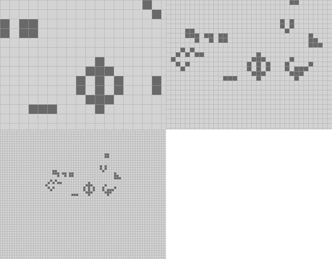
In the code for the previous episode the UI consisted just of a picture box that updated every second. The UI for this episode adds a new feature: you can now scroll with the mouse wheel to change the zoom level from cells being one pixel up to 64×64 pixels, in powers of two:

It’s just like scrolling in a map application; the current position of the mouse determines the center point for the zoom.

I’ve also made the default starting configuration a Life form called “acorn”, because it is very small and grows into a surprisingly large tree. It takes over 5000 ticks to settle down into a stable configuration and throws off a bunch of gliders as it does. The screen shots above are from the early stages in acorn’s evolution; check out the whole thing. It is quite mesmerizing. (Though you might want to adjust the timing in the code to compute more than two ticks per second!)


The first problem we face when designing a Life algorithm is the unavoidable fact that the board is in theory infinite, but our time and space available are finite. There are three basic ways to deal with this problem, and they all have their own pros and cons:

Fixed subset, dead everywhere else

Pick a board size: 256 x 256 cells, say. Everything outside the rectangle with corners (0, 0) and (255, 255) is considered permanently dead regardless of whether it really “ought” to be alive. We pick a size that is “big enough” for examining whatever Life form it is we wish to examine and do not worry about it further. If we end up with living cells near the border that would cause cells outside the border to come alive, we ignore that and they stay dead.

Fixed subset, wrap-around borders

Again, pick a finite size, treat everything outside that rectangle as permanently dead. But this time, make the board “wrap around” such that the “north” edge is adjacent to the “south” edge and the “east” edge is adjacent to the “west” edge.  If, say, a glider is heading towards the south edge, when it gets there it just keeps on going and appears on the north side of the rectangle.

There are two basic ways of conceptualizing this. The first and most common is that instead of an infinite flat grid, we’ve mapped a finite rectangular grid onto the surface of a torus — a doughnut. Imagine you took a rubber rectangle, rolled it into a cylinder to affix the north edge to the south edge, and then folded it to affix the now-circular west edge to the east edge. You’d end up with a torus.

The less common conceptualization is that we still have an infinite flat board, but we have tiled it with infinitely many copies of our rectangle; when we make a change to one tile, all the tiles change.

This technique is attractive from an implementation perspective because every cell has eight mutable neighbors and computing which cells are neighboring which others is simple math. However, it has a lot of problems too, particularly: if a Life form causes a glider to form that “escapes”, it ought to run off to infinity and bother no one again. But on a doughnut board it wraps around and ends up shooting straight at the cells that created it, possibly interfering with the evolution of the configuration.

We won’t be using this technique in this series.

Embiggen as needed

We start with a fixed subset that is as large as we need, but when we have a cell that might come alive on the border, we push the boundary out. There are a lot of clever ways to do this; our final algorithm in this series will use this idea to some extent.


Enough chit-chat; let’s look at the code for what I call the naïve algorithm. The basic idea is: create a 256×256 array of bools; true means alive, false means dead. On every tick, create a new array, check every cell’s neighbors in the old array to see if the cell will be alive in the next tick, and then discard the old array.

I’ll omit the boring boilerplate code.

Initialization is straightforward; the default state of a bool array is all false:

class BoolArrayLife : ILife
{
  private int height = 256;
  private int width = 256;
  private bool[,] cells;
  public BoolArrayLife()
  {
    Clear();
  }
  public void Clear()
  {
    cells = new bool[width, height];
  }

Everything outside our rectangle is always dead:

  private bool IsValidPoint(long x, long y) => 
    0 <= x && x < width && 0 <= y && y < height;

  public bool this[long x, long y]
  {
    get
    {
      if (IsValidPoint(x, y))
        return cells[x, y];
      return false;
    }

And similarly for the setter; you see how this goes.

To determine how many living neighbors a cell has, we just ask the indexer for the state of each neighbor. If the cell is out of range, the indexer tells us it is dead:

  private int LivingNeighbors(int x, int y)
  {
    int sum = this[x - 1, y - 1] ? 1 : 0;
    sum += this[x - 1, y] ? 1 : 0;
    sum += this[x - 1, y + 1] ? 1 : 0;
    sum += this[x, y - 1] ? 1 : 0;
    sum += this[x, y + 1] ? 1 : 0;
    sum += this[x + 1, y - 1] ? 1 : 0;
    sum += this[x + 1, y] ? 1 : 0;
    sum += this[x + 1, y + 1] ? 1 : 0;
    return sum;
  }

And the core “inner loop” algorithm — that is, what do we do on each tick? — is as straightforward as can be:

  public void Step()
  {
    bool[,] newCells = new bool[width, height];
    for (int y = 0; y < height; y += 1)
      for (int x = 0; x < width; x += 1)
      {
        int count = LivingNeighbors(x, y);
        newCells[x, y] = count == 3 || (cells[x, y] && count == 2);
      }
    cells = newCells;
  }

Recall that the client asks the engine to call it back for every living cell inside a certain rectangle. Were you ever asked the question “how do you compute the intersection of two rectangles?” in an interview? It’s a boring and clichéd question but sometimes you actually do need to loop over the intersection of two rectangles!

public void Draw(LifeRect rect, Action<LifePoint> setPixel)
{
  long xmin = Max(0, rect.X);
  long xmax = Min(width, rect.X + rect.Width);
  long ymin = Max(0, rect.Y - rect.Height + 1);
  long ymax = Min(height, rect.Y + 1);
  for (long y = ymin; y < ymax; y += 1)
    for (long x = xmin; x < xmax; x += 1)
      if (cells[x, y])
        setPixel(new LifePoint(x, y));
}

And that’s it! Just a bunch of loops.


Next time on FAIC: We’ll start exploring some of the questions that I want to discuss in this series, like:

  • What are the correctness and performance characteristics of this solution?
  • Are there easy ways we could reduce the computational burden?
  • How does it scale?
  • What can we learn about optimization in general from optimizing to solve this problem in particular?


Life, part 2

Code for this episode can be found here.


There are literally fifty years of articles explaining Conway’s Game of Life, starting with the one that introduced it to me: the October 1970 issue of Scientific American. Seems like a great time to do one more! I’ll go pretty quickly, since this is familiar to a lot of readers already.

Imagine an infinite flat board of square cells, like a huge piece of ordinary graph paper. Every cell has only two possible states, which we conveniently call “alive” and “dead”.

Just as the space in which Life is played is divided into discrete portions, so too is time. In the Life universe every time the clock “ticks”, some cells may be born, some may continue to live, and some may die. The rules governing this evolution are straightforward:

  • The “neighbors” of a cell are the eight cells which surround it.
  • If a cell is alive now and has exactly zero or one living neighbors, it dies of loneliness.
  • If a cell is alive now and has exactly two or three living neighbors, it survives.
  • If a cell is alive now and has four or more living neighbors, it dies from overcrowding.
  • If a cell is dead now and has exactly three living neighbors, it becomes alive.
  • If a cell is dead now and has any other number of living neighbors, it stays dead.

These rules can be simplified greatly; I leave it as an exercise to the reader to verify that these rules are the same:

  • If a cell has exactly three living neighbors then it is alive on the next tick irrespective of whether it is currently alive or dead.
  • Otherwise, if a cell is alive and has exactly two living neighbors then it is alive on the next tick.
  • Otherwise, the cell is dead on the next tick.

Let’s look at some simple examples:

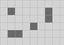
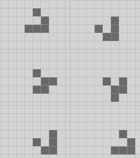
All of the living cells have one or no living neighbors, so they will all be dead on the next tick. Only one of the dead cells has exactly three living neighbors. On the next tick this will have a single living cell, and then on the tick after that they’ll all be dead.

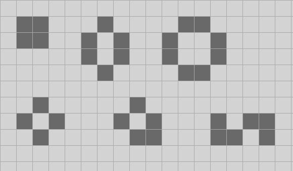
By contrast, these “still lifes” have the property that every living cell has two or three living neighbors, but no dead cell has exactly three living neighbors. These still lifes are traditionally called the block, beehive, pond, tub, boat and snake; they are stable. There are many, many more stable structures like this.

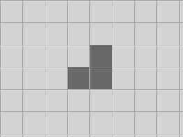
The easiest birth that leads to a stable configuration is this triomino:

I’m sure you see which dead cell has exactly three living neighbors; it will be alive in the next tick. All the live cells have two living neighbors, and no other dead cell has three, so this will turn into a block and then will be stable.

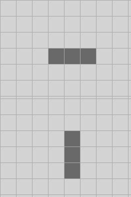
Can we come up with an oscillating pattern? It is not hard!

For obvious reasons this triomino is called “blinker”. There are a number of other relatively small configurations like this which oscillate with a period of two ticks.

I’ll finish this introduction off with the most important simple pattern in Life, the glider:

The glider oscillates between two basic forms, but after two ticks it has reflected itself along the diagonal axis, and then two ticks later it reflects back again to the original form, but offset by one cell “east” and one cell “south”. The glider is the simplest “spaceship” pattern; it is stable as it moves around the board. Here I’ve shown nine ticks in the life of a glider.

Clearly we can build gliders that move northeast, northwest and southwest easily enough, just by rotating the glider to “point” another direction.


I want to look at some different techniques for simulating Life. As will become extremely apparent when you look at the code or run the executable, I almost never write the user interface portion of any software package; my entire career I’ve built semantic analyzers for programming languages and there’s not a lot of UI design there. If I make foolish mistakes in my UI code, please feel free to point them out.

I’m therefore going to divide the project into a client form that has the user interface, that talks to a computation engine over an interface. I’ll point out a few features of the client here and there, but mostly we’ll concentrate on the computations.

As usual, I’ll put the code on GitHub and I’ll make a separate branch for each episode with new code. Sorry Mac users, it is a WinForms application.

The initial attempt here barely even has a user interface; it does not respond to user input except for the standard close, resize, and so on. But I’ve laid the groundwork for eventually implementing a more sophisticated client. In particular, a key problem to solve is identifying the rectangle of cells which is currently “in view” in the UI and rendering those cells to the UI. I’d like to be able to zoom in and out.

We could implement arbitrarily scaled zooming, but as we’ll see in later episodes, it’s going to be convenient to restrict scaling to powers of two, and as I said, I’m interested more in the algorithms than a pleasant UI.

In order to achieve this, an important bit of form state is:

 private int scale = -5;

The convention that I’m using here takes a moment to wrap your head around. The convention is:

  • If the scale is zero, then every on-screen pixel represents exactly one Life cell. This is implemented in the client, but since there is no control surface yet, you’ll have to adjust the scale in the debugger or recompile the code.
  • If the scale is a negative number, then we are “zoomed in”. Each Life cell is represented by a square that is 1 << -scale pixels wide. By default, I’ve set the scale to -5, which means that each Life cell is represented by a 32 by 32 square of pixels. Again, you can tweak that up or down in the debugger.
  • If the scale is a positive number then we go the other way: each pixel represents a square that is 1 << scale Life cells wide. This feature is not yet implemented, so don’t bump the scale up into positive numbers just yet.

A lot of the code in the form is about translating from the pixel-based bitmap coordinates, where (0, 0) is the upper left corner; the x coordinate increases to the right, and the y coordinate increases as we go down. The Life grid is an infinite plane where each cell can be addressed by a pair of integers, so there is no “corner”; I’m using the standard graph paper convention that the x coordinate increases to the right and the y coordinate increases as we go up. That entails some tricky bookkeeping, but we’ll manage. I’ve configured the UI so that when it starts up, Life coordinate (-2, -2) is in the lower left corner of the picture box.

I’ve introduced my own immutable point and rectangle structs to represent regions of the Life grid. That’s for three reasons. First, because the default point and rectangle structs are mutable, which gives me hives. Second, because they use integers, and I’m eventually going to be building Life grids that cannot be addressed by integers. And third, because as long-time readers of this blog know, I like to use the type system to find my mistakes before I make them. I’m not going to mix up LifePoint and Point easily!

The only other notable thing about the client is that it has a rarity; I’ve written unsafe code for something other than a compiler test case! That has happened only a handful of times in multiple decades of writing C# code. Setting individual pixels in a bitmap is slow and I’m going to be potentially setting a lot of them, so I’ve created a little function that parties directly on the raw bits of a bitmap in memory.

The interface between the client and the computation engine is straightforward; we’ll be making it more complex in later episodes as we add features to the client:

interface ILife
{
  void Clear();
  bool this[long x, long y] { get; set; }
  bool this[LifePoint v] { get; set; }
  void Draw(LifeRect rect, Action<LifePoint> setPixel);
  void Step();
}

This represents a mutable Life grid; long-time readers of my blog know that I prefer immutable data structures, and we’ll look at how to represent an immutable Life grid efficiently in later episodes. Fortunately it is almost always easy to make a mutable implementation on top of an immutable one, but often not easy to go the other way.

The two indexers are just for convenience; they are semantically identical.

The Clear and Step methods should be straightforward; one clears the board of all living cells, and Step moves the board forward one tick.  We’ll add methods in later versions to move forward multiple steps.

The Draw method is the interesting one. Basically the idea here is that Life boards almost always have far more dead cells than alive cells because the overcrowding rule tends to keep the density low. We can therefore get a win by only drawing the live cells.

The convention for drawing is: the client passes in the rectangular region of the board that the client wishes to render, and the engine calls the callback for every live cell. In order to implement the “zoom out” feature we’ll make this method a little more sophisticated in future versions, so that the engine only calls back once per “block of cells” that contains a live cell.


Next time on FAIC: We’ll look at the naive implementation of the engine and discuss its time and memory performance.


Life, part 1

Screen Shot 2020-04-13 at 8.54.56 AM.pngThe mathematician John Horton Conway has died, apparently due to the covid-19 epidemic, at the age of 82. I never met him but by all accounts, he was a delightful person and brilliant mathematician; his charming book on introductory game theory, Winning Ways, is the most fun you can have reading a university level math text. I had just purchased a biography, Genius at Play, before the crisis began and I suppose I’ll have time to read it now.
I’m sad, of course; we are all diminished when we lose a delightful and brilliant teacher. I’m also angry at the frankly disgusting attitude I see in the media and in the actions of elected officials that it is somehow no great loss to society when a disease predominantly kills the elderly. Scrooge’s they had better die and reduce the surplus population was meant to be taken as the horrifyingly Malthusian ranting of a bitter, foolish man who ought to know better, not as words to live by.

But I don’t intend this to be another rant as to the utter, abject, criminal stupidity that has informed the response to this pandemic. Rather: I have been wanting for over a decade to write a series on my blog about Conway’s most famous invention (I almost said discovery, because it seems like such a natural part of my world), Conway’s Game of Life. Now seems like a good time.

When I was a teenager I collected back issues of Scientific American — mostly from the sadly now gone Casablanca Books in my home town. Lots of the articles were interesting, but mostly I wanted a set of all the Martin Gardner, Kee Dewdney and Douglas Hofstadter’s monthly columns on mathematics and programming.


ASIDE: A note to any teenagers reading this who are collecting bulky old stuff like me. Keep it. When I moved across country I took my National Geographics and Tolkien biographies, but I sold my SciAms and Doctor Who novelizations for pennies on the dollar because they were bulky and I figured I wouldn’t miss them. And now only 25 years later I wish I still had those memorabilia.


I kept photocopies of Gardner’s articles on Life in 1970 and 1971 that introduced the phenomenon to the world. I find it fascinating to think about how Conway and the other people who made initial discoveries must have worked, without fast computers and fancy graphics; Conway said in the original 1970 article “it is marvelous to sit watching on the computer screen”, so there must have been some graphical system, but I can only imagine that it was quite primitive.

Over the next few weeks I’ll recapitulate my own experience with Life, though with much better hardware, software, and coding skills than my initial forays on my Amiga 500 as a teenager. We’ll start with the basics and work our way up to an astonishing result: it is possible to compute trillions of generations per second on Life boards with trillions of cells using an ordinary desktop computer.

I have learned recently that Conway did not consider Life to be the important work that he wanted to be remembered for — though I must say, if there’s something you don’t want to be remembered for, maybe don’t spend a decade popularizing it — but Life is for the ages; it will outlive us all. Early exposure to Life made me think about programming in ways I had not before, and I am grateful to John Conway for giving me and so many others that inspiration. I’ll leave it to my mathematical betters to remember his lasting contributions to professional mathematics.

Next time on FAIC: We’ll begin at the beginning with the rules of the game and some straightforward implementations.

Report thy feat unto Lord British

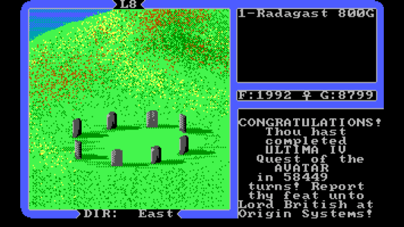
Welcome to yet another working-from-home pandemic episode of Fun For Friday Fabulous Adventures. Over the past while I’ve gradually been looking for music, movies and games I enjoyed as a teenager and seeing how they hold up. So I am pleased to announce that it took me only 35 years to finally complete a game I started on my Commodore 64 in 1985:

U4box.jpg

If you are unfamiliar with Ultima IV: it was an incredibly influential game that moved the state of the art forwards in “swords and sorcery” style games. The world was, for its time, enormously detailed, full of characters you could interact with who gave you clues as to the various puzzles you had to solve to win the game. Those puzzles largely took the form of “fetch quests” — you need eight magic stones hidden in six dungeons, and the mantras of eight shrines and the Bell of Courage, and so on; there’s quests built upon quests upon quests.

But the most interesting thing about Ultima IV was that it was the first game I played, and maybe the first game ever, to not just build in a moral system, but to make it the object of the game. The central design element is to not just reward, but require the player to be just, honest, compassionate, honorable and humble within the context of the game, and the quest is ultimately for wisdom. It was an astonishing achievement in a world where the object of all previous fantasy games was “kill the big bad guy”.

Other aspects of the game design are interesting by contrasting them to game design today. The game assumes, for example, that you have read the detailed (and well-produced) manuals that came in the box. It assumes that you’re reading the (cloth!) map and deciphering the runic lettering on it. This would not typically fly today; we expect games to introduce players gradually, to have a tutorial mode built into the game itself, and to not rely on anything exogenous to the software.

It’s a hard game to win without help. I remembered a great many details from my teenage years, and I knew that I could just look up all the mantras and locations of secret items and whatnot on the internet, but I decided to play it more or less like I did not have any of that information ahead of time. I did read some walkthroughs of the harder dungeon levels, because figuring out where all the secret door triggers are is tedious.

Ultima IV is available for free from GOG, and the rest of the series is cheap, so I encourage you to give it a shot if you want some of the retro gaming experience that informed modern fantasy game tropes.


Spoiler ahead:

If you do, there’s a bit of a cheat that I wish I’d remembered: once you are an Avatar and have the Mystic Robes, you can sell them, use the proceeds to buy magic wands and bows, and then find the robes again in the same place you found it the first time. That takes out a lot of the tedium of trying to get enough gold to afford magic ranged weapons. And don’t waste your money on magic armor; just get the Mystic Robes sooner rather than later!


The game ends with an exhortation to contact game author Lord British, also known as Richard Garriott, who amazingly is still making fantasy games that come with cloth maps in the box. I’ll have to order a copy and see how the series has evolved in the last 35 years.

Back in the 1980s if you did contact Lord British after winning an Ultima game, he would send you an autographed certificate of completion, but sadly I suspect I will not be getting one.

2020-04-06 (4).png

I also had Ultima V for my Amiga but I never got very far in it. Perhaps I’ll give it a shot next.