Code for this episode is here.

Today we can finish off our C# implementation of Stafford’s algorithm. Last time we turned the first pass into a table lookup; it might be a bit harder to optimize the second pass. Let’s take a look at the inner loop of the second pass; I’ll take out the comments and the debugging sanity checks:

Triplet t = triplets[x, y];
if (!t.Changed)
  continue;
if (t.LeftNext)
  BecomeAlive(x * 3, y);
else
  BecomeDead(x * 3, y);
if (t.MiddleNext)
  BecomeAlive(x * 3 + 1, y);
else
  BecomeDead(x * 3 + 1, y);
if (t.RightNext)
  BecomeAlive(x * 3 + 2, y);
else
  BecomeDead(x * 3 + 2, y);
changes.Add((x, y));

The key to understanding why this is very suboptimal is to look at what the code actually does in a common case. Let’s suppose the “current” triplet state is “dead-alive-alive” and the “next” triplet state is “alive-alive-dead”. That is, the left cell is going to become alive, the middle cell is going to stay alive, and the right cell is going to die.  What happens? Let’s go through it line by line.

if (!t.Changed)

Do some bit twiddling to discover that the current state and the next state are in fact different.

if (t.LeftNext)

Do some bit twiddling to discover that the next state is “alive”. Call BecomeAlive. What does it do?

if (t.LeftCurrent) return false;

Do some more bit twiddling to discover that yes, a change needs to be made.

triplets[tx - 1, y - 1] = triplets[tx - 1, y - 1].UUP();
triplets[tx, y - 1] = triplets[tx, y - 1].PPU();
triplets[tx - 1, y] = triplets[tx - 1, y].UUP();
triplets[tx, y] = t.SetLeftCurrent(true);
triplets[tx - 1, y + 1] = triplets[tx - 1, y + 1].UUP();
triplets[tx, y + 1] = triplets[tx, y + 1].PPU();

Do some bit twiddling to set the current bit to alive; do five additions to five neighbouring triplets to update their living neighbour counts — in parallel, for the cases where there are two counts to update — and return to the inner loop:

if (t.MiddleNext)

Do some bit twiddling to discover that the middle cell “next” state is alive, and call BecomeAlive:

if (t.MiddleCurrent) return false;

Do more bit twiddling to discover that the middle cell is already alive, so there’s no work to do. Go back to the inner loop:

if (t.RightNext)

Do some bit twiddling to discover that the right cell “next” state is dead; call BecomeDead:

if (!t.RightCurrent) return false;

Do some bit twiddling to discover that it is currently alive and so neighbour counts need to be updated.

triplets[tx, y - 1] = triplets[tx, y - 1].UMM();
triplets[tx + 1, y - 1] = triplets[tx + 1, y - 1].MUU();
triplets[tx, y] = t.SetRightCurrent(false);
triplets[tx + 1, y] = triplets[tx + 1, y].MUU();
triplets[tx, y + 1] = triplets[tx, y + 1].UMM();
triplets[tx + 1, y + 1] = triplets[tx + 1, y + 1].MUU();

Twiddle bits to set the current bit to dead; update the neighbour counts of five neighbouring triplets, two of which we just updated when we did the left cell!

Also, did you notice that when we did the left cell, we added one to the middle neighbour counts of the above and below triplets, and just now we subtracted one from that same count? We are doing work and then undoing it a few nanoseconds later.

The observations to make here are:

• On the good side, the idempotency check at the top of the algorithm is quite cheap. The cost of having duplicates on the “current changes” list is really low. But everything else is terrible.
• We are doing way too much bit twiddling still, and it is almost all in the service of control flow. That is, most of those bit twiddles are all in “if” statements that choose a path through the algorithm to selectively run different operations.
• If the left and right cells both changed then we need to update all eight neighbouring triplets, but we actually do ten updates.
• Worse, if the left, right and middle cells changed, we need to update eight neighbouring triplets but we actually would do twelve updates!
• We twiddle bits to set the current state up to three times, but we know what the final current state is going to be; it is the same as the “next” state.

How can we fix these problems?

The thing to notice here is there are only 27 possible control flows through this algorithm.They are:

• The idempotency check says that we already processed this change. Continue the loop.
• The left and middle cells are unchanged; the right cell is going from dead to alive.
• The left and middle cells are unchanged; the right cell is going from alive to dead.
• The left and right cells are unchanged; the middle cell is going from dead to alive.
• … and so on; you don’t need me to list all 27.

Let’s come up with a notation; I’ll say that “A” is “was dead, becomes alive”, “D” is “was alive, becomes dead”, and “U” is “no change”. The 27 possible control flows are therefore notated UUU, UUA, UUD, UAU, UAA, UAD, UDU, UDA, UDD, and so on, up to DDD. There are three positions each with three choices, so that’s three-to-the-three = 27 possibilities.

Since there are only 27 control flows, let’s just make a helper method for each! The control flow I just spelled out would be notated AUD, and so:

private bool AUD(int tx, int y)
{
  triplets[tx - 1, y - 1] = triplets[tx - 1, y - 1].UUP();
  triplets[tx, y - 1] = triplets[tx, y - 1].PUM();
  triplets[tx + 1, y - 1] = triplets[tx + 1, y - 1].MUU();
  triplets[tx - 1, y] = triplets[tx - 1, y].UUP();
  triplets[tx + 1, y] = triplets[tx + 1, y].MUU();
  triplets[tx - 1, y + 1] = triplets[tx - 1, y + 1].UUP();
  triplets[tx, y + 1] = triplets[tx, y + 1].PUM();
  triplets[tx + 1, y + 1] = triplets[tx + 1, y + 1].MUU();
  return true;
}

There are eight neighbouring triplets that need updating; we update all of them exactly once. We will see why it returns a bool in a minute.

You might be wondering what happens for something like “DDU” — left dies, middle dies, right unchanged. In that case there are neighbouring cells in other triplets that need to have their counts adjusted by two. We could write:

private bool DDU(int tx, int y)
{
  triplets[tx - 1, y - 1] = triplets[tx - 1, y - 1].UUM();
  triplets[tx, y - 1] = triplets[tx, y - 1].MMM().MMU();
  ...

But we notice here that we could save an addition by again, making the compiler fold the constant math:

private bool DDU(int tx, int y)
{
  triplets[tx - 1, y - 1] = triplets[tx - 1, y - 1].UUM();
  triplets[tx, y - 1] = triplets[tx, y - 1].M2M2M();
  ...

where we define a helper on the triplet struct:

public Triplet M2M2M() =>
  new Triplet(-2 * lcountone - 2 * mcountone - rcountone + triplet);

We can implement all 27 methods easily enough and we need 12 new helper methods to do the additions. These methods are all tedious, so I won’t labour the point further except to say that method UUU — no change — is implemented like this:

public bool UUU(int tx, int y) => false;

Meaning “there was no change”. All the other methods return true.

So it is all well and good to say that we should make one method for every workflow; how do we dispatch those methods?

We observe that there are only 64 possible combinations of current state and next state, and each one corresponds to one of these 27 workflows, so let’s just make another lookup; this one is a lookup of functions.

We will treat the current state as the low three bits of a six-bit integer, and the next state as the high three bits; that gives us our 64 possibilities. If, say, the next state is alive-alive-dead (AAD) and the current state is dead-alive-alive (DAA) then the change is “become dead-unchanged-become alive” (DUA):

lookup2 = new Func<int, int, bool>[]
{
  /* NXT CUR */
  /* DDD DDD */ UUU, /* DDD DDA */ UUD, /* DDD DAD */ UDU, /* DDD DAA */ UDD,
  /* DDD ADD */ DUU, /* DDD ADA */ DUD, /* DDD AAD */ DDU, /* DDD AAA */ DDD,
  /* DDA DDD */ UUA, /* DDA DDA */ UUU, /* DDA DAD */ UDA, /* DDA DAA */ UDU,
  /* DDA ADD */ DUA, /* DDA ADA */ DUU, /* DDA AAD */ DDA, /* DDA AAA */ DDU,
  /* DAD DDD */ UAU, /* DAD DDA */ UAD, /* DAD DAD */ UUU, /* DAD DAA */ UUD,
  /* DAD ADD */ DAU, /* DAD ADA */ DAD, /* DAD AAD */ DUU, /* DAD AAA */ DUD,
  /* DAA DDD */ UAA, /* DAA DDA */ UAU, /* DAA DAD */ UUA, /* DAA DAA */ UUU,
  /* DAA ADD */ DAA, /* DAA ADA */ DAU, /* DAA AAD */ DUA, /* DAA AAA */ DUU,
  /* ADD DDD */ AUU, /* ADD DDA */ AUD, /* ADD DAD */ ADU, /* ADD DAA */ ADD,
  /* ADD ADD */ UUU, /* ADD ADA */ UUD, /* ADD AAD */ UDU, /* ADD AAA */ UDD,
  /* ADA DDD */ AUA, /* ADA DDA */ AUU, /* ADA DAD */ ADA, /* ADA DAA */ ADU,
  /* ADA ADD */ UUA, /* ADA ADA */ UUU, /* ADA AAD */ UDA, /* ADA AAA */ UDU,
  /* AAD DDD */ AAU, /* AAD DDA */ AAD, /* AAD DAD */ AUU, /* AAD DAA */ AUD,
  /* AAD ADD */ UAU, /* AAD ADA */ UAD, /* AAD AAD */ UUU, /* AAD AAA */ UUD,
  /* AAA DDD */ AAA, /* AAA DDA */ AAU, /* AAA DAD */ AUA, /* AAA DAA */ AUU,
  /* AAA ADD */ UAA, /* AAA ADA */ UAU, /* AAA AAD */ UUA, /* AAA AAA */ UUU
};

We can extract the key to this lookup table from a triplet with a minimum of bit twiddling:

public int LookupKey2 => triplet >> 9;

And we need one final bit twiddle to set the current state to the next state:

public Triplet NextToCurrent() => 
  new Triplet((triplet & ~currentm) | ((triplet & nextm) >> 3));

Put it all together and our second pass loop body is greatly simplified in its action, though rather harder to understand what it is doing:

int key2 = triplets[x, y].LookupKey2;
Func<int, int, bool> helper = lookup2[key2];
bool changed = helper(x, y);
if (changed)
{
  triplets[x, y] = triplets[x, y].NextToCurrent();
  changes.Add((x, y));
}

We determine what work needs to be done via table lookup; if the answer is “none”, the helper returns false and we do nothing. Otherwise the helper does two to eight additions, each updating one to three neighbour counts in parallel. Finally, if necessary we update the current state to the next state and make a note of the changed triplet for next time.

We’re down to a single control flow decision, and almost all the bit operations are simple additions, so we will likely have considerably improved performance.

It was a long road to get here. I sure hope it was worth it…

Algorithm           time(ms)  ticks  size(quad)    megacells/s
Naïve (Optimized):   4000       5K      8               82
Abrash                550       5K      8              596
Abrash w/ changes     190       5K      8             1725 
Abrash, O(c)          240       5K      8             1365
Stafford v1           340       5K      8              963
Stafford v2           210       5K      8             1560
Stafford final        180       5K      8             1820

A new record for this series, so… yay?

Also, it is still an O(change) algorithm, and it is significantly more space-efficient at three cells per two bytes, instead of one cell per byte, so that’s good; we can store larger grids in the same amount of memory if we want.

But oh my goodness, that was a lot of work to get around a 25% speedup over the one-byte-per-cell O(change) algorithm.

Reading Abrash’s original article from the 1990s describing Stafford’s algorithm, it is a little difficult to parse out exactly how fast it is, and how much faster that is than Abrash’s original algorithm. If I read it right, the numbers are approximately:

• 200×200 grid of cells
• 20MHz-33MHz 486
• Measure performance of the computation, not the display (as we are also doing)
• Roughly 20 ticks per second for Abrash’s O(cells) “maintain neighbour counts” algorithm.
• Roughly 200 ticks per second for Stafford’s O(changes) implementation.

Dave Stafford attained a 10x speedup by applying optimizations:

• Store the next state, current state, and neighbour counts in a triplet short
• Maintain a deduplicated change list of previously-changed triplets
• Table lookup to compute next state of possibly-changed triplet
• Branch to a routine that does no more work than necessary to update neighbour counts

Obviously machines are a lot faster 25 years later. Stafford’s algorithm running on a 20MHz 486 does 200 ticks per second, and the same algorithm written in C# running on a 2GHz i7 does over 25000 ticks per second even with a 50%+ larger grid size. But we should expect that a machine with 100x clock speed, better processor caches, and so on, should do on the order of 100x more work per second.

(Aside: though we are doing 65536 cells in a grid instead of their 40000, Abrash and Stafford’s implementations also implemented wrap-around behaviour for the edges, which I have not; that complicates their implementations and I avoided the penalty of writing code to deal with those complications. So this is not a purely apples-to-apples comparison in many ways.)

What is a little surprising here is: my implementation of the two algorithms in C# shows a 3x speedup between the two algorithms that were originally compared, not a 10x speedup as was original observed.

Figuring out why exactly would require rather more analysis of the original code than I’m willing to do, but I have a few conjectures.

First, we don’t know what the test case was. If it had a small number of changes per tick then certainly an O(changes) algorithm is potentially much better than an O(cells) implementation. Perhaps the test case was biased towards O(changes) algorithms.

Second, I have implemented the spirit of both algorithms but there are a lot of differences. My favourite, by way of example, is that Stafford’s original machine code implementation does not use a lookup array for the second-pass optimization, like I do here. The triplet value itself (with some bits masked out) is the address of the code that is invoked. Let me repeat that in case it was not clear: it’s machine code so you have total authority to decide where in memory the helper functions are, and they are placed in memory such that the triplet itself is a pointer to the helper function. There is no table indirection penalty because there is no table.

These are the sorts of tricks that machine language programmers back in the 1990s lived for, and though I can admire it, that’s just not how we do stuff in high level languages. We could spend a bunch of time tweaking the C# versions of these algorithms to use pointers instead of offsets, or arrays with high water marks instead of lists, and so on. We’d get some wins, but they’d be marginal, and I’m not going to bother tuning this further. (As always, if anyone wants to, please make the attempt and leave a comment!)

The third conjecture is: yes, the rising tide of a 100x processor speed improvement lifted all boats, but it also changed the landscape of performance optimization because not all code is gated on processor speed. RAM latency, amount of available RAM, cache sizes, and so on, have also changed in that time but not at the same rate, and not to the same effect. Figuring out whether any of those changes had the effect of bringing these two algorithms’ performance closer together in the last 25 years is really hard to say.

Next time on FAIC: I want to do some experiments to look more directly at the scalability of these algorithms; do costs actually grow as O(change)? What happens if we make some larger grids where lots of stuff is changing?

Coming up after that: Every algorithm we’ve looked at so far uses some sort of two-dimensional array as the backing store, which limits us to grids that are, in the grand scheme of things, pretty small. Can we come up with storage solutions that are less constrained, and at what performance cost?

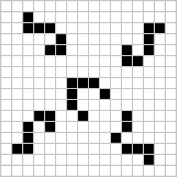
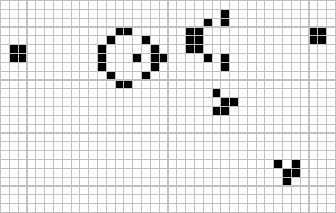
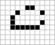
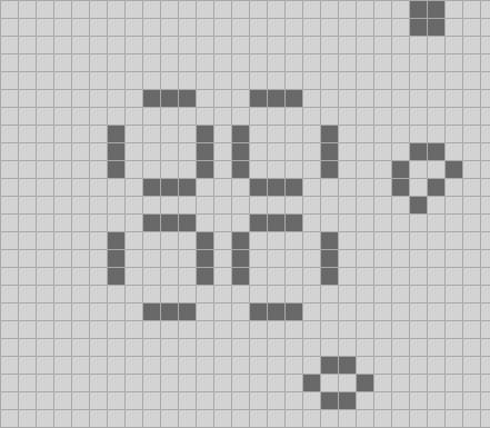
For today’s extra content: a puffer whose debris is spaceships is called a rake; the first rake discovered back in the 1970s is called spacerake. (Image from the wiki.)

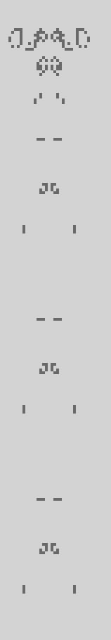
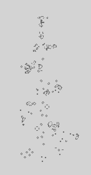
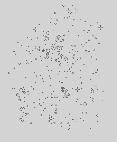
Again we see that you can do interesting things by sticking a bunch of c/2 spaceships together. Here’s a wider view snapshot that maybe makes it a little more clear how it comes to resemble “raking” the plane:

And again, this is an example of a pattern which causes the number of changes per tick to grow linearly over time.

Code for this episode is here.

A couple episodes back we did a first cut at implementing Stafford’s algorithm using the triplet data structure to store the current and upcoming states of three cells and their living neighbour counts, all in 15 bits of a 16 bit short. Unsurprisingly, it was quite a bit slower than the same algorithm that did one byte per cell; any win from parallelism is swamped by, I conjectured, all the extra bit twiddling.

Is there a way to eliminate some of that bit twiddling?

Today we’ll look at the inner loop of the first pass, which identifies cells that need to change by setting their next state bits:

Triplet c = triplets[x, y];
Triplet t = c;
int lc = t.LeftCount;
int mc = t.MiddleCount;
int rc = t.RightCount;
t = t.SetLeftNext(lc == 3 | t.LeftCurrent & lc == 2);
t = t.SetMiddleNext(mc == 3 | t.MiddleCurrent & mc == 2);
t = t.SetRightNext(rc == 3 | t.RightCurrent & rc == 2);
if (t.Changed)
{
  currentChanges.Add((x, y));
  triplets[x, y] = t;
}

What essentially are we doing here?

• Compute the new triplet t from the old triplet c.
• If t is different than c, cause two side effects: update an array, and update a list.

There’s nothing we can do about the side effects, but we can observe that the computation has the following characteristics:

• We compute the left, middle and right actual counts; each does bit twiddling to extract one or two states, and one three-bit integer, and then some addition.
• We then do bit twiddling to again extract the three states…
• and then we do a bunch of comparison logic on all of the above
• The net result is the three “next state” bits, which we again use bit twiddling to get into place in the new triplet.
• And, cherry on top, we do a bunch of bit twiddling to extract the current and next state bits to ask “was there a change?”
• Oh, the pain.

We have a function that consumes 12 bits of a 16 bit short and produces a new 16 bit short and a Boolean saying whether it changed. But given those 12 bits, the short and the Boolean produced are always the same. We can precompute the results for every possible input once and look them up as our inner loop.

That is, we can move the vast majority of the bit twiddling backwards in time to before the algorithm runs the first step.

We will need a lookup key containing the twelve bits we need; fortunately, they are the bottom twelve bits so we can extract them with a minimum of bit twiddling by adding a helper to the triplet struct:

public int LookupKey1 => triplet & 0x0fff;

I’ll create two lookups, one for “will there be a change?” and one for “what is the new triplet?” Since the lookups are keyed on a 12-bit integer, we can simply make them both arrays; there’s no need for anything fancier:

static class TripletLookup
{
  public static Triplet[] lookup;
  public static bool[] changed;

and initialize them in a static constructor; we just create every possible triplet based on the bottom 12 bits, and compute what the inner loop of the first pass did in the previous version:

  static TripletLookup()
  {
    lookup = new Triplet[1 << 12];
    changed = new bool[1 << 12];
    for (int left = 0; left < 2; left += 1)
      for (int middle = 0; middle < 2; middle += 1)
        for (int right = 0; right < 2; right += 1)
          for (int lc = 0; lc < 8; lc += 1)
            for (int mc = 0; mc < 7; mc += 1)
              for (int rc = 0; rc < 8; rc += 1)
              {
                Triplet t = new Triplet()
                  .SetLeftCurrent(left == 1)
                  .SetMiddleCurrent(middle == 1)
                  .SetRightCurrent(right == 1)
                  .SetLeftCountRaw(lc)
                  .SetMiddleCountRaw(mc)
                  .SetRightCountRaw(rc)
                  .SetLeftNext(
                    (lc + middle == 3) | (left == 1) & (lc + middle == 2))
                  .SetMiddleNext(
                     (left + mc + right == 3) | (middle == 1) & (left + mc + right == 2))
                  .SetRightNext(
                    (middle + rc == 3) | (right == 1) & (middle + rc == 2));
                lookup[t.LookupKey1] = t;
                changed[t.LookupKey1] = t.Changed;
              }
  }

And that’s that.

A few things to note here. First, honestly, how often are you justified in writing a six-deep nested loop? Not very often, so let’s take the opportunity while we’ve got it!

Second, a great many of these lookup conditions are impossible. In Life you cannot get into a situation where the middle cell of a triplet has seven living neighbours that are not left or right, AND left and right both have zero living neighbours other than the middle. Who cares? These two tables take up 12KB of memory, total. We can waste some. And the cost of doing the unnecessary calculations is only paid once, at startup.

Moreover, in Stafford’s original implementation he went even further and did not bother to pull out the twelve bits for the key; he just precomputed the entire triplet-to-triplet function and made a table with 65536 entries. Why do any bit twiddling at all?

Anyway, we can now replace the entire inner loop of the first pass with:

int key1 = triplets[tx, y].LookupKey1;
if (TripletLookup.changed[key1])
{
  triplets[tx, y] = TripletLookup.lookup[key1];
  currentChanges.Add((tx, y));
}

So much nicer to read, and much faster. Let’s once again run 5000 generations of acorn on an 8-quad:

Algorithm           time(ms)  ticks  size(quad)    megacells/s
Naïve (Optimized):   4000       5K      8               82
Abrash                550       5K      8              596
Abrash w/ changes     190       5K      8             1725 
Abrash, O(c)          240       5K      8             1365
Stafford v1           340       5K      8              963
Stafford v2           210       5K      8             1560

We are back in business! We have a three-cells-per-short O(c) algorithm that beats the one-cell-per-byte O(c) algorithm and is within striking distance of beating the “copy the array every time” version.

Aside: I told a small fib earlier in this episode; did you catch it?

Give that some thought and then scroll down.

.

.

.

.

.

.

.

…we can move the vast majority of the bit twiddling backwards in time to before the algorithm runs the first step.

I put my fib in boldface for added foolery.

When exactly does the lookup initialization happen? I worked on the compiler team and the language design team and I still always have to double-check Jon’s page on the subject whenever it comes up.

Since we have a static class with a static constructor, the static constructor will run when a member is accessed for the first time; we are not using the “relaxed” semantics. That means: the cost of precomputing the tables is incurred during the first call to Step, not before. This could make a difference to our performance metrics!

It does not, because when I collected those metrics I ensured that Step had already been called at least once before I started the stopwatch. But I had to know to do that.

Incidentally, the purpose of the “relaxed” semantics is to allow the initialization of the static fields to happen when the first method that accesses those fields is jitted. That way the jitter does not have to emit code to ensure that the fields are initialized; it just initializes them and then it knows they are initialized! I’ve always found it a little ironic that the “relaxed” semantic means that the jitter gets more eager about calling the initializers early. More eagerness seems like an odd thing to characterize as “relaxed”.

Next time on FAIC: Optimizing the first pass was pretty straightforward. Optimizing the second pass is maybe not so easy. We will do so, and finish up our exploration of Stafford’s algorithm.

For today’s extra content: last time I mentioned that a common technique is to use eaters to constrain unwanted expansion of some pattern in an oscillator; this has been used for a long time, as evidenced by two oscillators discovered in 1972 by Robert Wainwright: dinner table, and roteightor. (Images from wiki; see links.)

Code for this episode is here.

We’ll take a short break from getting to our C# version of Stafford’s algorithm; in this episode I want to talk about some improvements to the UI, and also talk about some more fundamental interesting Life patterns.

The basic loop for the UI is pretty simple: compute and display one tick on every timer event. We have no problem keeping up with one tick every 30 milliseconds. Let’s say just to keep the numbers nice and round that we’re running at 32 ticks per second.

Obviously we could go a lot faster; with the 8-quads we’ve been playing with thus far we can go many hundreds of times faster. We could render every other generation, or every fourth generation, or heck, every 1024th generation, 32 times a second.

I’m going to use the same logarithmic scale that I’ve been using for grid sizes — recall, an n-quad is a square with side 2-to-the-n — and apply it to time as well. That is, speed 0 means “go forward one tick”.  Speed 1 means “go forward two ticks”.  Speed 2 is four ticks, speed 3 is eight ticks, and so on.

For the UI, what we’ll do is use this same convention; speed 0 is one tick per second, speed 1 is two ticks per second, and so on.  As an implementation detail, for speeds 0 through 5 — one per second through 32 per second — we will instruct the algorithm to step forward a single tick, and control the update speed by changing the timer duration. Once we get above speed 5, we will set the timer to update 32 times a second, and have the algorithm loop to compute a (speed – 5) block of ticks.

If you look at the code it will probably make sense. Give it a shot and play around a bit with the speed controls, see how you like it.

If you do look at the code you might notice that the looping code has been copied into the algorithm classes a half a dozen times, rather than putting it in the UI code once. The reason why will become clear later on in this series.

On that mysterious note, let’s leave speed control aside and talk about guns that shoot spaceships.

A few episodes back we were discussing patterns that grow without bound; I said that there were two questions you could ask about spaceships that would illuminate the existence of such patterns:

• Are there puffers? That is, spaceships that leave a trail of debris, stable or unstable, behind? We saw that yes, there are, and therefore there are patterns that add cells forever if allowed room to do so.
• Are there oscillators that stay in one place but regularly shoot out spaceships? If so, then the spaceship gun will lead to a continued growth of live cells as more and more spaceships fly away.

Based on our discussion so far it should come as no surprise that both the first puffers and the first guns were discovered by Bill Gosper in 1970. Here’s a simple oscillator called the “queen bee shuttle” — so called because the queen bee here is trying to build a hive, which is then immediately destroyed because it gets too close to the block. The queen bee does a U turn and promptly does the same thing on the other side, giving us a 30-tick oscillator:

(Images from the wiki.)

The queen bee behaviour when not captured between blocks leads to stable debris in 191 ticks. It is pleasant to watch evolve, so check that out; I’ve added a pattern file to the branch for this episode.

But the astonishing thing is: if you make two overlapping queen bee shuttles, you get a surprise:

Every 30 ticks we get a new glider, forever. This was the first Life pattern discovered that was known to exhibit unbounded growth. Moreover, there is a lot we can do with an infinite supply of spaceships. We’ll come back to discuss a few of those things in a future episode.

Right now though I want to highlight a more recently constructed glider gun, just because I think it’s neat. This is the AK-94 glider gun; it produces two gliders going opposite directions every 94 ticks, though the variant shown here “eats” the northwest-bound glider rather than allowing it to escape.

(For reasons unknown, WordPress refuses to display the animated version of this graphic; see the link above to the wiki for an animated version.)

The “fish hook”-like still Lifes you see all over this pattern are called, well, fish hooks by some people, but the more usual name is eater 1— so named because it was the first simple pattern discovered that survives being hit by a lot of stuff. It is therefore very useful in construction of purpose-built Life patterns because it eats cells that would otherwise grow into unwanted chaos and eats gliders that you do not want escaping for whatever reason.

Once again we have seen that there are patterns that exhibit linear growth; as the number of ticks increases, the number of cells that are changing every tick also increases as an O(n) function of time, so any O(change) algorithm is going to get slower over time. However we still have not answered the question “are there patterns that have a superlinear growth of living cells over time?” Keep pondering that!

A great many more spaceship guns have been constructed, and some of them have interesting properties. However I think I will leave it there for now, and get back to our exploration of Stafford’s algorithm.

Next time on FAIC: How can we use our “triplet” data structure to optimize the inner loop of the first phase of the step algorithm, where we compute the “next state” bits?

Source code for this episode is here.

We are continuing with our project to gradually morph Abrash’s “remember the living neighbour counts” algorithm into Stafford’s algorithm. I’m going to start today by adding two very small bit-twiddling optimizations to the Triplet wrapper struct I introduced in the previous episode.

The first optimization is: I’m going to need to update neighbour counts, but remember, we’re going to be updating a short with three neighbour counts in it. Let’s look at an example of a 3×3 grid represented by three shorts, and assume that every other cell in the larger grid is dead.

I’ll give the current state as “A” for alive, “D” for dead, and the counts are “raw” counts; that is, the left-hand living neighbour counts are not including the state of the middle cell, and the middle neighbour counts are not including the left or right cells, and so on.

The scenario is that an L-shaped triomino is about to become a block:

        Before                  After
        A-1  A-1  D-0           A-2  A-2  D-1
        A-2  D-2  D-1   ==>     A-2  A-2  D-1
        D-1  D-1  D-0           D-2  D-2  D-1

What has to happen? The middle triplet’s living neighbour counts do not need to change. But when the middle-of-the-middle triplet cell becomes alive, we need to increase all three living neighbour counts by one in both the upper and lower triplet.

Suppose the middle triplet is in a rectangular array of triplets at x, y. We do not want to have to write for this scenario:

n = triplet[x, y - 1];
triplets[x, y - 1] = n.SetLeftCountRaw(n.LeftCountRaw+1)
                      .SetMiddleCountRaw(n.MiddleCountRaw+1)
                      .SetRightCountRaw(n.RightCountRaw+1);
s = triplet[x, y + 1];
... oh the boredom ...

That’s both tedious and unnecessarily slow because of all the bit twiddling. Instead I’m going to write 15 helper functions as follows:

private const int lcountone = 1 << lcount;
private const int mcountone = 1 << mcount;
private const int rcountone = 1 << rcount;
public Triplet UUP() => new Triplet(rcountone + triplet);
public Triplet UUM() => new Triplet(-rcountone + triplet);
public Triplet UPU() => new Triplet(mcountone + triplet);
public Triplet UPP() => new Triplet(mcountone + rcountone + triplet);
public Triplet UMU() => new Triplet(-mcountone + triplet);
public Triplet UMM() => new Triplet(-mcountone - rcountone + triplet);
public Triplet PUU() => new Triplet(lcountone + triplet);
public Triplet PUM() => new Triplet(lcountone - rcountone + triplet);
public Triplet PPU() => new Triplet(lcountone + mcountone + triplet);
public Triplet PPP() => new Triplet(lcountone + mcountone + rcountone + triplet);
public Triplet MUU() => new Triplet(-lcountone + triplet);
public Triplet MUP() => new Triplet(-lcountone + rcountone + triplet);
public Triplet MMU() => new Triplet(-lcountone - mcountone + triplet);
public Triplet MMM() => new Triplet(-lcountone - mcountone - rcountone + triplet);

To add one to a three-bit integer embedded inside a short, all we need to do is add one shifted to the right position in the short! We do not need to extract the bits, put them in an integer, do the arithmetic, and then put them back.

(Also, fun bonus nano-optimization: since I put the constants on the left, the ones with multiple operations will get folded at compile time.)

The naming is of course P for plus, M for minus, U for unchanged; the operation I described above would be “PPP”.

The second optimization is: I want to be able to quickly answer the question “is anything going to change in this triplet on this tick?” What we’re going to do, recall, is set three “next state” bits, so the answer to my question is: are the next-state bits as an integer equal to the current-state bits as an integer? If the answer is yes, then there was no change.

private const int currentm = lcm | mcm | rcm;
private const int nextm = lnm | mnm | rnm;
public int CurrentState => (currentm & triplet) >> rcur;
public int NextState => (nextm & triplet) >> rnext;
public bool Changed => CurrentState != NextState;

All right, let’s get into it. The basic layout of the class is by design almost exactly the same as our previous algorithm because that’s the whole idea of this pedagogy:

class StaffordOne : ILife
{
  private int height = 258;
  private int width = 88;
  private Triplet[,] triplets;
  private List<(int, int)> changes;

We have a rectangular array of 258×88 triplets. The top and bottom row, and the left and right triplet will be a rectangle of death, so that gives us 256×258 cells to play with.

The change list coordinates are triplet array coordinates, not Life grid coordinates.

I’ve still got my “BecomeAlive” and “BecomeDead” helper methods. They take Life grid coordinates. They are still idempotent but they no longer update the change list because I want to do that on a per-triplet granularity, not a per-cell-changed granularity, and I don’t want to use a hash table to deduplicate the change list.

Rather, they return true or false, changed or unchanged, and let the caller decide how to update the change list.

private bool BecomeAlive(int x, int y)
{
  int tx = x / 3;
  Triplet t = triplets[tx, y];
  switch (x % 3)
  {
  case 0:
    if (t.LeftCurrent)
      return false;
    triplets[tx - 1, y - 1] = triplets[tx - 1, y - 1].UUP();
    triplets[tx, y - 1] = triplets[tx, y - 1].PPU();
    triplets[tx - 1, y] = triplets[tx - 1, y].UUP();
    triplets[tx, y] = t.SetLeftCurrent(true);
    triplets[tx - 1, y + 1] = triplets[tx - 1, y + 1].UUP();
    triplets[tx, y + 1] = triplets[tx, y + 1].PPU();
    break;

As in Abrash’s algorithm, we do the expensive work of updating the living neighbour counts only when something changed. If the left cell in a triplet changed then we need to update the counts of the triplets to the north, south, west, northwest and southwest.

We don’t need to update the count of the middle cell in the current triplet because changing the state of the left state bit is what is going to update that count.

And we do not need to update the counts of the triplets to the east, northeast or southeast because those triplets have no neighbours in common with the left cell of this triplet.

I’m going to omit the middle and right cells; you see how this goes I’m sure. And the “become dead” logic is all the same with the signs inverted so let’s skip that too.

The real business logic is in the step function. As before, we do it in two passes.

In the first pass we look at every triplet on the previously-changed list and the neighbour triplets of all those triplets, which might include duplicates. We make a “current changes” list of every triplet that is going to change, and stash that change in the “next” bits of the triplet.

In the second pass we update the neighbour counts and current state bits of every changed cell. As we do so, we create a deduplicated changes list for the next tick.

public void Step()
{
  var currentChanges = new List<(int, int)>();
  foreach ((int cx, int cy) in changes)
  {
    int minx = Max(cx - 1, 1);
    int maxx = Min(cx + 2, width - 1);
    int miny = Max(cy - 1, 1);
    int maxy = Min(cy + 2, height - 1);
    for (int y = miny; y < maxy; y += 1)
    {
      for (int x = minx; x < maxx; x += 1)
      {

This is basically the same code as before, but something to note here. Suppose we have a triplet that is on the “changed” list because its left cell, and only its left cell, changed on the previous tick. We are now examining the neighbouring triplets, which includes the northeast, east and southeast neighbouring triplets, but those are not affected by a change in the left cell. We are therefore frequently doing unnecessary work here. Isn’t this bad?

There are ways to avoid that, but as we keep adding optimizations to our implementation of Stafford’s algorithm, we’ll see that it becomes very cheap to process a neighbour that is not going to change. In cases where it is more expensive to run an “avoidable work detector” than it is to simply do the work, it’s better to do the work. I’m therefore going to ignore this small problem for the remainder of the exploration of the algorithm.

Now we get into the meat of the algorithm, as usual:

        Triplet c = triplets[x, y];
        Triplet t = c;
        int lc = t.LeftCount;
        int mc = t.MiddleCount;
        int rc = t.RightCount;
        t = t.SetLeftNext(lc == 3 | t.LeftCurrent & lc == 2);
        t = t.SetMiddleNext(mc == 3 | t.MiddleCurrent & mc == 2);
        t = t.SetRightNext(rc == 3 | t.RightCurrent & rc == 2);
        if (t.Changed)
        {
          currentChanges.Add((x, y));
          triplets[x, y] = t;
        }
      }
    }
  }
  changes.Clear();

That gets us through the first pass. The second pass is rather more verbose than our previous version because it is doing three cells per loop iteration, but is logically the same.

  foreach ((int x, int y) in currentChanges)
  {
    Triplet t = triplets[x, y];
    if (!t.Changed)
      continue;
    bool changed = false;
    if (t.LeftNext)
      changed |= BecomeAlive(x * 3, y);
    else
      changed |= BecomeDead(x * 3, y);
    if (t.MiddleNext)
      changed |= BecomeAlive(x * 3 + 1, y);
    else
      changed |= BecomeDead(x * 3 + 1, y);
    if (t.RightNext)
      changed |= BecomeAlive(x * 3 + 2, y);
    else
      changed |= BecomeDead(x * 3 + 2, y);
    Debug.Assert(changed);
    changes.Add((x, y));
  }
}

The changed flag I’m tracking there is just a cheap sanity check to make sure we’re not doing unnecessary work, and that BecomeAlive/BecomeDead are doing the right thing.

That’s it; rather more tedious code but the same algorithm as previous. We should expect that there is a performance penalty as we have added a bunch of bit twiddling that we did not have before but have only gained a very small amount of parallelism, like setting three neighbour counts with a single addition. If we run the performance test on the release build we get:

Algorithm           time(ms)  ticks  size(quad)    megacells/s
Naïve (Optimized):   4000       5K      8               82
Abrash                550       5K      8              596
Abrash w/ changes     190       5K      8             1725 
Abrash, O(c)          240       5K      8             1365
Stafford v1           340       5K      8              963

We’ve lost almost half the speed of our previous best version of this algorithm. I sure hope there was a point to all this.

Next time on FAIC: We’ll take another brief foray into some interesting Life forms, and improve the speed controls in the client.

Coming up after that: How can we optimize the heck out of the first pass inner loop given this data structure?

For today’s extra content: the creepiest spaceship, Spider:

Image from the wiki.

Code for this episode is here.

Where were we? I was gradually changing Abrash’s “remember the neighbour counts” into Stafford’s algorithm from an early 1990s optimization contest. In this series I’m going to illustrate the algorithm in C#, and we’ll conjecture along the way how the performance characteristics are different from the original machine language implementation; I’m more interested in the ideas expressed in the algorithm than the exact implementation details.

So far we’ve got:

• Each cell takes six bits out of a byte; one for its current state, four for the count of its neighbours, and one to express the “new state” for a cell that is changing.
• We create a “previous changes” list for use on the next tick; by checking whether the “new state” and “current state” bits are the same, we make adding to the change list idempotent, and thereby deduplicate it.
• The tick algorithm is O(changed cells).

Dave Stafford’s observation was that if we can compress “six bits per cell” down to five, then we can store three cells in a 16 bit short. That doesn’t sound like a win, but in a few episodes we will see why it is — maybe.

A brief aside: when I ask technical interview questions I always try to base them on a problem I actually had to solve in the real job. Back in the day we needed to make sure that VBScript could work on 64 bit Windows machines; it previously had only been compiled to 16 and 32 bit Windows. (Yes, 16 bit; Internet Explorer ran on Windows 3.1 in 1996 when I started on the scripting team.) We immediately ran into a problem that, full disclosure, I had caused.

You see, VBScript used the VARIANT data structure internally to store data, and VARIANT had an unused 32 bit field in the middle of it that I was using to stash a pointer to some supplemental data. The trouble is: the 64 bit version of VARIANT still only had a 32 bit unused field, so we could not stash a pointer in there anymore. So… now what? That’s the problem I had to solve.

The interview question was a simplified version of this scenario, and let me tell you, the number of candidates who tried to store 64 pounds of bits in a 32 pound sack boggled the mind. So I will forgive you if you’re skeptical right now that there is a way to compress six bits down to five!

How then to do this impossible thing? The key observation is that the reason we need four bits for the living neighbour count is because there are nine possibilities: zero through eight living neighbours. If we only needed to represent eight possibilities then we could do it in three bits. Without further ado, we’re going to store three cells in a 16 bit short like this:

• Call the three cells Left, Middle and Right, or L, M, R for short.
• Bit 15 is unused; the original implementation did “wrap around” behaviour and used this bit to store whether the triplet was on an edge or not. I’m going to instead continue to use a “surrounding rectangle of death” approach.
• Bits 14, 13 and 12 are the “next state” of L, M, and R.
• Bits 11, 10 and 9 are the “current state” of L, M and R.
• Bits 8, 7 and 6 are a three-bit integer giving the count of living neighbours of Left that are not Middle; we already know the state of Middle in bit 13.
• Bits 5, 4 and 3 are a three-bit integer giving the count of living neighbours of Middle that are not Right or Left.
• Bits 2, 1 and 0 are similarly the living neighbour count of Right not counting Middle.

And that’s how we fit 18 pounds into a 15 pound sack.

As usual in this series and in life, I’m going to make an immutable value type that wraps a short and put all the bit twiddling code in methods of the struct:

struct Triplet
{
  private short triplet;
  public Triplet(short triplet)
  {
    this.triplet = triplet;
  }
  // Bit numbers
  private const int lnext = 14;
  private const int mnext = 13;
  private const int rnext = 12;
  private const int lcur = 11;
  private const int mcur = 10;
  private const int rcur = 9;
  private const int lcount = 6;
  private const int mcount = 3;
  private const int rcount = 0;

  // Bit masks
  private const int lnm = 1 << lnext;
  private const int mnm = 1 << mnext;
  private const int rnm = 1 << rnext;
  private const int lcm = 1 << lcur;
  private const int mcm = 1 << mcur;
  private const int rcm = 1 << rcur;
  private const int lcountm = 7 << lcount;
  private const int mcountm = 7 << mcount;
  private const int rcountm = 7 << rcount;

  // Getters and setters
  // I'm going to want the state as both integers and bools because
  // I do math on them.
  public bool LeftNext => (lnm & triplet) != 0;
  public bool MiddleNext => (mnm & triplet) != 0;
  public bool RightNext => (rnm & triplet) != 0;

  public int LeftNextRaw => (triplet & lnm) >> lnext;
  public int MiddleNextRaw => (triplet & mnm) >> mnext;
  public int RightNextRaw => (triplet & rnm) >> rnext;

  public Triplet SetLeftNext(bool b) =>
    new Triplet(b ? (lnm | triplet) : (~lnm & triplet));
  public Triplet SetMiddleNext(bool b) =>
    new Triplet(b ? (mnm | triplet) : (~mnm & triplet));
  public Triplet SetRightNext(bool b) =>
    new Triplet(b ? (rnm | triplet) : (~rnm & triplet));

  public bool LeftCurrent => (lcm & triplet) != 0;
  public bool MiddleCurrent => (mcm & triplet) != 0;
  public bool RightCurrent => (rcm & triplet) != 0;

  public int LeftCurrentRaw => (triplet & lcm) >> lcur;
  public int MiddleCurrentRaw => (triplet & mcm) >> mcur;
  public int RightCurrentRaw => (triplet & rcm) >> rcur;

  public Triplet SetLeftCurrent(bool b) =>
    new Triplet(b ? (lcm | triplet) : (~lcm & triplet));
  public Triplet SetMiddleCurrent(bool b) =>
    new Triplet(b ? (mcm | triplet) : (~mcm & triplet));
  public Triplet SetRightCurrent(bool b) =>
    new Triplet(b ? (rcm | triplet) : (~rcm & triplet));
  // I want to be able to access both the raw bits and the logical count.
  public int LeftCountRaw => (lcountm & triplet) >> lcount;
  public int MiddleCountRaw => (mcountm & triplet) >> mcount;
  public int RightCountRaw => (rcountm & triplet) >> rcount;

  public int LeftCount => 
    MiddleCurrentRaw + LeftCountRaw;
  public int MiddleCount => 
    LeftCurrentRaw + RightCurrentRaw + MiddleCountRaw;
  public int RightCount => 
    MiddleCurrentRaw + RightCountRaw;

  public Triplet SetLeftCountRaw(int c)
  {
    Debug.Assert(0 <= c && c <= 7);
    return new Triplet((c << lcount) | ~lcountm & triplet);
  }
  public Triplet SetMiddleCountRaw(int c)
  {
    Debug.Assert(0 <= c && c <= 6);
    return new Triplet((c << mcount) | ~mcountm & triplet);
  }
  public Triplet SetRightCountRaw(int c)
  {
    Debug.Assert(0 <= c && c <= 7);
    return new Triplet((c << rcount) | ~rcountm & triplet);
  }
}

Well, that was a little tedious, but it will make the rest of the code read less like bit twiddling.

You know what, I think that is enough for today; the ideas in Stafford’s algorithm are interesting but the amount of code you have to write, as we’ll see, it’s a lot.

Next time on FAIC: We’ll implement the algorithm we have so far — rectangular array of cells, rectangle of death, remembering neighbour counts, change list, store next state in the cell — using the Triplet data structure instead. Unsurprisingly, the added bit twiddling is not cheap; will it pay for itself by unlocking an additional optimization? Stay tuned!

For today’s extra content: the prettiest spaceship, the Canada Goose. Image from the wiki.

You’ll note that it is a glider that “pulls along” a pattern behind it that would not otherwise be a spaceship in itself; this situation is called a “tagalong”. There are also “pushalongs” where the spaceship extension goes in the front.

Source code for this episode is here.

Before we get into today’s episode proper, a quick note. I’ve updated the client so that it now supports the ability to load a pattern off disk, execute that pattern, and “reset” back to the start state. I’ve also included files for every pattern I’ve mentioned so far in this series, and will continue to add them as future episodes progress.

There are a great many standard formats for Life patterns and I’ve made quick-and-dirty parsers for the two most common; the details are not particularly interesting or clever, so I won’t go into them here.

We’ve been looking at algorithms for quite some time now, and we’re making good progress. We can compute 5000 ticks of the evolution of “acorn” in around 200 milliseconds, which is not too shabby. But we haven’t looked at any patterns in particular other than the glider and acorn and a few common still lifes and oscillators. Today I thought I’d spend a little time on other spaceships.

A “spaceship” in Life is a pattern which oscillates but ends up offset from its original position. The first spaceship discovered was the glider, which moves diagonally one square every four ticks.

A natural question to ask is: how fast is that? We’ve seen during our optimizations so far that we can take advantage of the fact that a changed cell can only affect its immediate neighbours on the next tick; cells “two away” or more from the nearest changed cell cannot “feel” the effect of the change for at least that many ticks.

The analogy in the real world is of course the speed of light. If a star explodes ten thousand light years away, we have absolutely no way of knowing until ten thousand years later.

We therefore can characterize spaceship speed as a fraction of the maximum theoretically possible speed, which would be one cell per tick. Call that speed “c”, for obvious reasons. A glider has speed c/4. If the fraction has a numerator other than one, it is traditionally written before the c; a spaceship that moved two cells every five ticks would move at 2c/5.

I’ve gotten ahead of myself slightly here though; are there even any spaceships other than the glider? And do any move orthogonally, instead of diagonally?

I give you the heavyweight, middleweight and lightweight spaceships: (Images from the wiki.)

These are period-four c/2 orthogonal spaceships discovered by Conway in 1970, and of course you can point them in any of four directions, just like gliders.

There is a whole theory of spaceships in Life, which I might discuss some aspects of in future episodes; it includes topics like:

• Given simple spaceships, can we construct larger spaceships from them? As we’ll see later in this episode, simple spaceships can be combined in interesting ways.
• What happens when two or more spaceships collide? How can we vary the timing and direction of the collision to create debris that has interesting properties?
• Can we make spaceships that travel on “oblique” angles, other than orthogonal or diagonal? I was surprised to learn that the first oblique spacecraft was constructed only ten years ago, and the first “knightship” — that travels two-up-one-over — was discovered in 2018.
• and so on.

A question came up in the comments a few episodes back on the subject of “why do we care how big a grid we can compute in a reasonable time budget?” To start answering that question, let’s pose another question: are there any patterns that grow without bounds? When coming up with the initial rules for Life, one of Conway’s stated goals was to find a rule for how cells change where it was not initially obvious whether there was a pattern that constantly created new living cells. In the original 1970 SciAm article it was still not known, but by the follow-up three months later it was known that there were such patterns.

One way to attack that problem is to restrict it to a problem involving spaceships. If there is an oscillator that produces a spaceship as a side effect of its oscillation then it is a “spaceship gun”, and thus the population will grow forever. And similarly, if there is a “puffer” spaceship that produces immortal “debris” or “ash” in its wake as a side effect as it travels, then similarly the population will grow forever.

Bill Gosper, whose name is going to continue to come up a lot in this series, found both the first gun and the first puffer. We’ll come back to the gun later. The first discovered puffer is two slightly modified heavyweight spaceships traveling in tandem with some stuff between them:

The initial pattern is symmetric so the evolution will be symmetric as well. As this puffer travels it leaves behind debris which quickly settles down into a repeated pattern: four blinkers and the still life called “bookends”:

It does not take at all long to see that this grows without bound, and that the output is periodic in both space and time, and stable.

So far I have not made the case why we need large boards with fast computation. But now I give you the second puffer:

This time we have two modified lightweight spaceships with stuff between them, but now the pattern is not symmetrical and so there is no requirement that the output be either. I encourage you to load this one up in the client, but if you can’t run it, I’ll give some screen shots. I have an 8-quad grid — 256×256 — and I start the puffer close to the bottom edge.

Two things are immediately apparent. First, the output is completely chaotic. Second, as the wave of unstable debris grows, it intersects the “always dead” edge of the board and starts behaving differently than it would on a truly unbounded grid.

Keep on going:Regions of stability have started to emerge with common still life patterns including one and a half “honey farms” — four beehives in a cross. But it is not clear whether the chaotic region will spread back towards it or not, and new chaos is constantly being produced by the puffer.

The question now is: will the new chaos that is constantly being produced lead to a debris trail that remains chaotic forever? Or will it settle down into a stable oscillating pattern at some point? Will it be like an expanding plume? Will it be a column of spacially-repeating still lifes? Unclear at this point.

These questions are not easy to answer analytically, and are complicated by the fact that we do not know if the chaotic region is going to produce one or more gliders aimed back at the debris! Gliders can travel through the empty space between the still lifes, eventually hitting one of them and triggering a new chaotic front.

Let’s keep running until the puffer hits the wall of death at the top end of the quad:

It’s looking like some additional order has started to emerge; there seems to be a pattern of still lifes surrounding “traffic lights” — four blinkers arranged in a cross — that alternates left to right. So maybe there is hope that this settles down into something stable.

But since the puffer is now gone, we have lost our ability to determine the long-term behaviour of this pattern because there is no longer a source of new chaos coming in from the top. Regardless, we can let it run for a while anyways and see what happens on our 8-quad. A few ticks later, in the chaotic region to the lower left…

… we see one of those internal gliders I mentioned before. It ends up moving the blinkers around, removing the hive and adding a block, but does not spread chaos further.

A few hundred ticks later:

The initial honey farm that I pointed out has been half eaten. The top part of the grid is mostly stable but the middle is still chaotic and there is no evidence of any repeating pattern left in the debris. If we let it keep running then in a few thousand cycles it settles down to just still lifes, blinkers, and a few escaped gliders that hit the wall of death and turn into blocks.

This is a completely distorted picture of the real behaviour of the puffer caused by there being a wall of death near the bottom, where it began, and at the top, where the puffer was destroyed shortly after it was created.

Can we determine the real behaviour of this pattern? If we bump up the size of the grid to a 10-quad and make plenty of space at the top and bottom, we can easily see the true long-term behaviour.

Here’s what the bottom half of Puffer 2 actually looks like after the original chaos settles down when run on a sufficiently large grid. (You’ll have to edit the source code to see this one yourself, or wait until a future episode.)

The chaos being produced at the top by the puffer actually does not propagate too far down the debris field left behind before it dies out, and so the resulting ash is a nicely repeating pattern of still lifes and blinkers.

We started with a 22 cell configuration, but it took us doing computations on a 1024 by 1024 grid — which is a megabyte in our implementation — to get a good sense of its long-term behaviour. Imagine trying to do these sorts of analyses with 1970s-era hardware and you can see why there was so much interest in faster algorithms!

Aside: all the oscillators in the debris field are blinkers except for one that appears very late in the initial debris; did you spot it?

That is a “natural” occurrence of one of my favourite oscillators, the period-three pulsar; it was mentioned in the original 1970 SciAm article.

It is all very interesting to know that there are patterns like this which cannot be easily analyzed without a big board; are there other performance implications?

There certainly are!

• Both puffers produce arbitrarily many blinkers behind them as they run
• Therefore, the number of blinkers can grow linearly as a function of time
• Therefore, any algorithm that is O(change) on every tick is going to get slower and slower over time, as more and more blinkers are added.

Two questions to ponder:

• Any ideas on what to do about that?
• At least these puffers just add oscillating patterns linearly as a function of time. Are there puffers that add patterns which change, but as some other function of time? Quadratically, say? (That is, they add one oscillator, then four, then nine… growing as the square as time increases.)

Next time on FAIC: We’ll get back into gradually modifying Abrash’s algorithm that stores neighbour counts into Stafford’s algorithm that won Abrash’s optimization contest in the early 1990s. We will start by looking at the data structure that underlies this algorithm; it seems to be trading a large amount of bit twiddling for a small win in space, but the value will become clear eventually!