About ericlippert

http://ericlippert.com

Bean Machine Retrospective, part 4

Did I actually build a compiler? Yes and no.

Traditionally we think of a compiler as a program which takes as its input the text of a program written in one language (C#, say), and produces as its output an “equivalent” program written in another language (MSIL, say).  A more modern conception is: a compiler is a collection of code analysis services, and one of those services is translation.

I made a great many assumptions when embarking on this project. Some of the more important ones were as follows:

Assumption: we must implement everything necessary for a source-to-source translation, but that is not enough. The primary use case of Beanstalk is outputting samples from a posterior, not outputting an equivalent program text. Translation may be a secondary use case, but we will not succeed by stopping there.

We’re building a compiler in order to build a better calculator.

Static and dynamic analysis

Traditional translating compilers such as the C# compiler perform a “static” analysis of the code; that is, they analyze only (1) the text of the program and (2) metadata associated with already-compiled artifacts such as libraries. The code is not executed in a static analysis.

“Dynamic” analysis is by contrast an analysis of code while the code is running. 

Assumption: correct static analysis of Python is impossible for at least two reasons. 

1) Python is an extremely dynamic language; it is difficult to definitively know what any program identifier refers to, for example, without actually running the program to find out.

2) The model may depend upon non-stochastic model elements that are unknowable by static analysis. Model parameters or observed values can (and will!) be read from files or queried from databases, and those values must be present in the graph that we deduce.

We must build a dynamic analyzer; we’re going to run a modified version of the model code to find out what it does.

Pure functions, acyclic graph

For our purposes we define a pure function as one that:

  • Always terminates normally; it does not go into an infinite loop or throw an exception
  • Is idempotent: it always produces the same output when given the same input
  • Its action does not depend on mutating global state
  • Its action does not mutate global state

Examples of impure functions are easily produced:

mean = 1.0
@random_variable
def normal():
  global mean
  mean = mean + 1.0 # UH OH
  return Normal(mean, 1.0)

Or, just as bad:

mean = tensor([1.0])
@random_variable
def normal():
  global mean
  mean[0] += 1.0
  return Normal(mean, 1.0)

Assumptions:

  • Model builders will write pure functions. In particular, model builders will not mutate a tensor “in place” such that the mutation causes a change of behaviour elsewhere in the model
  • Beanstalk is not required to detect impure functions, though it may
  • Beanstalk may memoize model functions

Also: a Bayesian network never has cycles; the distribution of each node depends solely on the distributions of its ancestor nodes.

Assumptions:

  • Model builders will write models where no random variable depends upon itself, directly or indirectly.
  • Beanstalk is not required to detect cycles (though in practice, it does)

Note that a model may contain recursion if the recursion terminates. This is legal:

@random_variable
def normal(n):
  if n <= 0:
    mean = 0.0
  else:
    mean = normal(n-1)
  return Normal(mean, 1.0)
queries = [ normal(0) ]
observations = { normal(2): tensor(0.0) }

Next time on FAIC: Having made these and other assumptions, I embarked upon an implementation. But before I can explain the implementation, I should probably answer some nagging questions you might have about what exactly that random_variable decorator does.

Bean Machine Retrospective, part 3

Introducing Beanstalk

Last time I introduced Bean Machine Graph, a second implementation of the PPL team’s Bayesian inference algorithm. We can compare and contrast the two implementations:

  • BMG emphasizes mechanisms; BMG programs are all about constructing a graph. BM emphasizes business logic
  • A point which I did not emphasize yesterday but which will come up again in this series: BMG requires many node constructions be annotated with semantic types like “probability” or “positive real”. BM lacks all “type ceremony”.
  • BMG programs represent operations such as addition as verbose calls to node factories. BM concisely represents sums as “x + y ”, logs as “x.log()”, and so on

In short, the BMG user experience is comparatively not a great experience for data scientists, in the same way that writing in machine code is not great for line-of-business programmers. We wished to automatically convert models written in Bean Machine into equivalent programs which constructed a graph, and then got the improved inference performance of BMG.

OK… how?

A program which translates one language to another is called a compiler, and that’s where I came in. We code named the compiler “Beanstalk”. I started working on Beanstalk in October of 2019 given this brief:

Construct a compiler which takes as its input a Bean Machine model, queries and observations, and deduces from it the equivalent BMG graph (if there is one).

If we can solve that problem effectively then we get the best of both worlds. Data scientist users can write models using a pleasant Python syntax easily integrated into their existing PyTorch workflows, but get the inference performance afforded by BMG. The “concept count” — the number of APIs that the data scientist must understand — increases only slightly, but their workflows get faster. That is a win all around.

Does it work today?

Yes. Barely. If for some strange reason you want to play around with it, you can obtain the code from github. The error messages are terrible, the compiler is “over fit” to specific models that we needed to get compiled, and it is quite slow, but for simple models it does work. At the time the team was shut down we were actively extending both BMG and the compiler to handle more general models efficiently.

Early on we realized that of course the compiler is a means to an end, not an end in itself. What users really wanted was a more efficient inference engine that just happened to use BMG as its back end, so that’s the main API. You can call BMGInference().infer(), passing in queries, observations, and so on, just like any other Bean Machine inference engine; the compiler will analyze the source code of the queries, produce a graph, and call BMG’s inference engine to produce samples from the queries posteriors.

It has a few other useful APIs as well that are more like a traditional source-in-source-out compiler.

  • BMGInference().to_graph() produces a graph object without starting inference.
  • BMGInference().to_python() and to_cpp() produce Python and C++ source code fragments which construct the graph.
  • BMGInference().to_dot() produces a program in the DOT graph visualization language; that’s what I used to make the graph diagrams in this series.

Next time on FAIC: What were my initial assumptions when tasked with writing a “compiler” that extracts a graph from the source code of a model? And is it really a compiler, or is it something else?

Bean Machine Retrospective, part 2

Introducing Bean Machine Graph

Bean Machine has many nice properties:

  • It is integrated with Python, a language often used by data scientists
  • It describes models using the rich, flexible pytorch library
  • Inference works well even on models where data is stored in large tensors

I’m not going to go into details of how Bean Machine proper implements inference, at least not at this time. Suffice to say that the implementation of the inference algorithms is also in Python using PyTorch; for a Python program it is pretty fast, but it is still a Python program.

We realized early on that we could get order-of-magnitude better inference performance than Bean Machine’s Python implementation if we could restrict values in models to (mostly) single-value tensors and a limited set of distributions and operators.

In order to more rapidly run inference on this set of models, former team member Nim Arora developed a prototype of Bean Machine Graph (BMG).

BMG is a graph-building API (written in C++ with Python bindings) that allows the user to specify model elements as nodes in a graph, and relationships as directed edges. Recall that our “hello world” example from last time was:

@random_variable
def fairness():
  return Beta(2,2)

@random_variable
def flip(n):
  return Bernoulli(fairness())

That model written in BMG’s Python bindings would look like this: (I’ve omitted the queries and observations steps for now, and we’ll only generate one sample coin flip instead of ten as in the previous example, to make the graph easier to read.)

g = Graph()
two = g.add_constant_pos_real(2.0)
beta = g.add_distribution(
  DistributionType.BETA,
  AtomicType.PROBABILITY,
  [two, two])
betasamp = g.add_operator(OperatorType.SAMPLE, [beta])
bern = g.add_distribution(
  DistributionType.BERNOULLI,
  AtomicType.BOOLEAN,
  [betasamp])
flip0 = g.add_operator(OperatorType.SAMPLE, [bern])

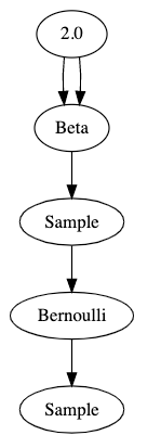
That’s pretty hard to read. Here’s a visualization of the graph that this code generates:

These graphs are properly called Bayesian network diagrams, but for this series I’m just going to call them “graphs”.


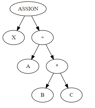
I should say a little about the conventions we use in this graphical representation. Compiler developers like me are used to decomposing programs into abstract syntax trees. An AST is, as the name suggests, a tree. ASTs are typically drawn with the “root” at the top of the page, arrows point down, “parent nodes” are above “child nodes”, and operators are parents of their operands. The AST for something like x = a + b * c would be

where X, A, B, C are identifier nodes.

Bayesian network diagrams are just different enough to be confusing to the compiler developer. First of all, they are directed acyclic graphs, not trees. Second, the convention is that operators are children of their operands, not parents.

The best way I’ve found to think about it is that graphs show data flow from top to bottom. The parameter 2.0 flows into an operator which produces a beta distribution — twice. That distribution flows into a sample operator which then produces a sample from its parent distribution. That sampled value flows into an operator which produces a Bernoulli distribution, and finally we get a sample from that distribution.

If we wanted multiple flips of the same coin, as in the original Python example, we would produce multiple sample nodes out of the Bernoulli distribution.


BMG also has the ability to mark sample nodes as “observed” and to mark operator nodes as “queried”; it implements multiple inference algorithms which, just like Bean Machine proper, produce plausible samples from the posterior distributions of the queried nodes given the values of the observed nodes. For the subset of models that can be represented in BMG, the performance of the inference algorithms can be some orders of magnitude faster than the Bean Machine Python implementation.

Summing up: Our team had two independent implementations of inference algorithms; Bean Machine proper takes as its input some decorated Python methods which concisely and elegantly represents models in a highly general way using PyTorch, but the inference is relatively slow. Bean Machine Graph requires the user to write ugly, verbose graph construction code and greatly restricts both the data types and the set of supported operators, but uses those restrictions to achieve large inference speed improvements.


Next time on FAIC: Given the above description, surely you’ve guessed by now what the compiler guy has been doing for the last three years on this team full of data scientists! Can we automatically translate a Bean Machine Python model into a BMG graph to get BMG inference performance without sacrificing representational power?

Bean Machine Retrospective, part 1

As I mentioned in the previous episode, the entire Bean Machine team was dissolved; some team members were simply fired, others were absorbed into other teams, and some left the company. In this series I’m going to talk a bit about Bean Machine and my work on what is surely the strangest compiler I’ve ever written.

I should probably recap here my introduction to Bean Machine from what now seems like an eternity ago but was in fact only September of 2020.

We also have some tutorials and examples at beanmachine.org, and the source code is at github.com/facebookresearch/beanmachine.


We typically think of a programming language as a tool for implementing applications and components: games, compilers, utilities, spreadsheets, web servers, libraries, whatever. Bean Machine is not that; it is a calculator that solves a particular class of math problems; the problems are expressed as programs.

The purpose of Bean Machine is to allow data scientists to write declarative code inside Python scripts which represents relationships between parts of a statistical model, thereby defining a prior distribution. The scientist can then input real-world observations of some of the random variables, and queries on the posterior distributions. That is, we wish to give a principled, mathematically sound answer to the question: how should we update our beliefs when given real-world observations?

Bean Machine is implemented as some function decorators which modify the behavior of Python programs and some inference engines which do the math. However, the modifications to Python function call semantics caused by the decorators are severe enough that it is reasonable to conceptualize Bean Machine as a domain specific language embedded in Python.


The “hello world” of Bean Machine is: we have a mint which produces a single coin; our prior assumption is that the fairness of the coin is distributed somehow; let’s suppose we have reason to believe that it is drawn from beta(2,2).

@random_variable
def fairness():
  return Beta(2,2)

We then flip that coin n times; each time we call flip with a different argument represents a different coin flip:

@random_variable
def flip(n):
  return Bernoulli(fairness())

We then choose an inference algorithm — say, single-site Metropolis — say what we observed some coin flips to be, and ask for samples from the posterior distribution of the fairness of the coin. After all, we have much more information about the fairness of the coin after observing some coin flips than we did before.

heads = tensor(1)
tails = tensor(0)
samples = bm.SingleSiteAncestralMetropolisHastings().infer(
    queries=[fairness()],
    # Say these are nine heads out of ten, for example.
    observations={ flip(0) : heads, [...] flip(9): tails },
    num_samples=10000,
    num_chains=1,
)

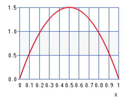
If we then did a histogram of the prior and the posterior of fairness given these observations, we’d discover that as the number of samples increased, the histograms would conform more and more closely to these graphs:

Prior: Beta(2,2)

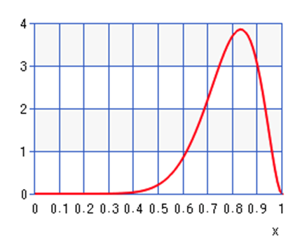
Posterior if we got nine heads and one tail in the observations:

When we observe nine heads out of ten, we should update our beliefs about the fairness of the coin by quite a large amount.

I want to emphasize that what this analysis gives you is not just a point estimate — the peak of the distribution — but a real sense of how tight that estimate is. If we had to make a single guess as to the fairness of the coin prior to observations, our best guess would be 0.5. In the posterior our best guess would be around 0.83. But we get so much more information out of the distribution! We know from the graphs that the prior is extremely “loose”; sure, 0.5 is our best guess, but 0.3 would be entirely reasonable. The posterior is much tighter. And as we observed more and more coin flips, that posterior would get even tighter around the true value of the fairness.

Notice also that the point estimate of the posterior is not 0.9 even though we saw nine heads out of ten! Our prior is that the coin is slightly more likely to be 0.8 fair than 0.9 fair, and that information is represented in the posterior distribution.


All right, that’s enough recap. Next time on FAIC: I’m not going to go through all the tutorials on the web site showing how to use Bean Machine to build more complex models; see the web site for those details. Rather, I’m going to spend the rest of this series talking about my work as the “compiler guy” on a team full of data scientists who understand the math much better than I do.

Life, part 38

Here we go again!

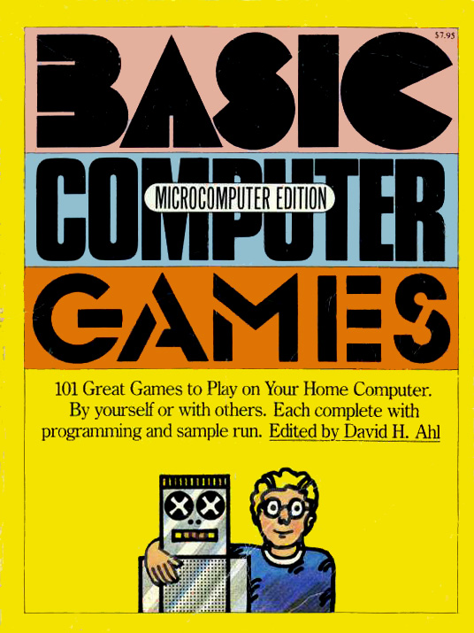
Fellow BASIC enthusiast Jeff “Coding Horror” Atwood, of Stack Overflow and Discourse fame, has started a project to translate the programs in the 1978 classic BASIC Computer Games into more modern languages. I never had a copy of this one — my first computer book was Practise Your BASIC — but these programs are characteristic of the period and I am happy to help out.

graphic of page

1978 was of course well into the craze of writing Life simulators for home personal computers. In this episode I’ll break down the original program assuming that you’re not a BASIC old-timer like me; this language has a lot of quirks. You can read the commentary from the book here, and f you want to run the original program yourself the copy here is a valid Vintage BASIC program.

Let’s get into it!

2 PRINT TAB(34);"LIFE"
4 PRINT TAB(15);"CREATIVE COMPUTING  MORRISTOWN, NEW JERSEY"
6 PRINT: PRINT: PRINT
8 PRINT "ENTER YOUR PATTERN:"
  • All lines are numbered whether they need to be or not. Line numbering is often used to indicate program structure; we’ll come back to this in a bit.
  • Lines are not one-to-one with statements! A single line may contain several statements separated by colons.
  • PRINT takes a semicolon-separated list of zero or more expressions.
  • PRINT outputs a newline by default; as we’ll see presently, there is a way to suppress the newline.
  • TAB(x) does not produce a string; it moves the “print cursor” to column x. In many versions of BASIC, TAB can only appear as an argument to PRINT.
9 X1=1: Y1=1: X2=24: Y2=70
10 DIM A(24,70),B$(24)
20 C=1
  • Variable names are typically one or two characters.
  • 24 x 70 is the size of the Life board that we’re simulating here; this was quite a large screen by 1978 standards. I owned both a Commodore 64 and a Commodore PET with 40×25 character screens; it was possible to get an 80-column PET but they were rare.
  • Note that the authors have made the bizarre choice throughout that (X, Y) coordinates refer to (line, column) and not the more standard (column, line) interpretation. Normally we think of X as being the left-right coordinate, not the top-bottom coordinate.
  • Single-valued variables need not be declared.
  • Array-valued variables are “dimensioned”, and the dimensions typically must be literal constants. Here we have a two-dimensional array and a one-dimensional array.
  • Anything that is string-valued has a $ suffix, so B$ is an array of strings.
  • Arrays and strings are both indexed starting from 1.
  • As we know from early episodes in this series, a naïve implementation needs to keep track of both the “current” and “next” state. In a memory-constrained environment such as can be assumed by a 1978 BASIC program’s author, we need to keep all that in the same array. Spoiler alert: the convention used by this program for the contents of array A is:
    • 0 means cell is dead, will stay dead.
    • 1 means cell is alive, will stay alive.
    • 2 means cell is alive, will die.
    • 3 means cell is dead, will come alive.
  • You might have noticed that the program is formatted to have very few unnecessary spaces. Having become accustomed to vertical and horizontal whitespace being used to reduce eyestrain and guide the reader, it looks dense and hard to read. This was not a stylistic choice though; it was imposed by the limitations of the technology of the time. Line lengths were constrained, often to the width of the screen, and when you have only 40 or 80 characters of screen, unnecessary spaces are bad. But more interesting from my perspective as a compiler writer is that implementations of BASIC often tokenized as the user typed in the program, and then stored only the tokens in memory, not the original source code as it was typed. When the program was listed back, the program printer reconstituted the program from the token stream which had discarded the spaces. Pre .NET versions of VB did this!
30 INPUT B$(C)
40 IF B$(C)="DONE" THEN B$(C)="": GOTO 80
50 IF LEFT$(B$(C),1)="." THEN B$(C)=" "+RIGHT$(B$(C),LEN(B$(C))-1)
60 C=C+1
70 GOTO 30
  • INPUT takes a string from the console and places it in the given variable.
  • Arrays are indexed using parentheses.
  • This is a “while” loop but most BASICs did not have loop structures beyond FOR/NEXT, or even ELSE clauses for IF/THEN statements. You had to write GOTO statements to build those control flows, as shown here. Notice that all the colon-separated statements execute if the condition of the IF is met; otherwise we continue on to the next statement. (I was fortunate to have access to an original PET with Waterloo Structured BASIC which did have while loops, though I did not understand the point of them when I was in elementary school. Many years later I ended up working with some of the authors of Waterloo BASIC in my first internships at WATCOM, though I did not realize it at the time! The whole saga of Waterloo Structured BASIC and the SuperPET hardware is told here.)
  • LEFT$, RIGHT$ and LEN do what they say on the tin: give you the left substring of given length, right substring of given length, and length of a string. Strings are not directly indexable.
  • + is both the string concatenation operator and the arithmetic addition operator.
  • It seems clear that we are inputting strings and sticking them in an array until the user types DONE, but why are we checking whether the first character in the string is a period, and replacing it with a space? It is because in some versions of BASIC, INPUT strips leading spaces, but they are necessary when entering a Life pattern.
  • Did you notice that nothing whatsoever was explained to the user of the program except “enter your pattern”? Enter it how? Why should the user know that spaces are dead, leading spaces are soft, a period in the first place is a hard space but a live cell anywhere else, and that you type DONE when you’re done? The assumption of the authors is that the only person running the code is the person who typed it in. “You should explain as little as possible” is not a great attitude to drill into beginner programmers.
  • Notice that we have no bounds checking. B$ was dimensioned to 24 elements; if the user types in more than 24 lines in the pattern, the program crashes. Similarly we have no checks on the lengths of the strings themselves. A whole generation of young programmers was taught from their very first lesson that crashes are the user’s fault for doing something wrong.
  • Our program state by the time we break out of the loop is: B$ has C lines in it, and B$(C) is an empty string.
80 C=C-1: L=0
90 FOR X=1 TO C-1
100 IF LEN(B$(X))>L THEN L=LEN(B$(X))
110 NEXT X
  • Since the last line is always blank, we are reducing the line count C by one.
  • The maximum line length L is initialized to zero, unnecessarily. I prefer an unnecessary but clear initialization to the lack thereof. But as we’ll see in a moment, some variables are just assumed to be initialized to zero, and some are initialized twice needlessly. More generally, programs that were designed to teach children about programming were chock full of sloppy inconsistencies and this is no exception.
  • FOR/NEXT is the only structured loop in many early BASICs. The loop variable starts at the given value and executes the body unless the loop variable is greater than the final value. Some versions of the language also had an optional STEP clause, and some would even keep track of whether the loop was counting up or down. Fancy!
  • Plainly the purpose of the FOR/NEXT loop here is to find the maximum line length of the pattern input by the user, but it appears to have a bug; we have strings in B$ indexed from 1 through C, but we are skipping the length check on B$(C). The subtraction here appears to be a mis-edit; perhaps the C=C-1 was moved up, but the developer forgot to adjust the loop condition. The bug only affects inputs where the last line is also the longest.
  • Is it inefficient to compute LEN(B$(X)) twice in the case where the maximum length L needs to be updated? Many versions of BASIC used length-prefixed strings (as do all versions of VB and all .NET languages) and thus computing length is O(1). When I first learned C as a teenager it struck me as exceedingly weird that there was no out-of-the-box system for length-prefixing a string. And it still does.
120 X1=11-C/2
130 Y1=33-L/2
140 FOR X=1 TO C
150 FOR Y=1 TO LEN(B$(X))
160 IF MID$(B$(X),Y,1)<>" " THEN A(X1+X,Y1+Y)=1:P=P+1
170 NEXT Y
180 NEXT X
  • There are no comments in this program; it would be nice to explain that what we’re doing here is trying to center the pattern that the user has just typed in to the interior of a 24 x 70 rectangle. (X1, Y1) is the array coordinate of the top left corner of the pattern as it is being copied from B$ to A; spaces are kept as zero, and non-spaces become 1. This automatic centering is a really nice feature of this program.
  • Once again we have no bounds checking. If L is greater than 67 or C is greater than 23, bad things are going to happen when we index into A. (Though if C is greater than 23, we might have already crashed when filling in B$.)
  • We already initialized X1 and Y1; we have not read their values at any point before they are written for a second time. By contrast, the population count P is accessed for the first time here and is assumed to be initialized to zero. Again, there is some amount of sloppiness going on here that could have been easily removed in code review.
200 PRINT:PRINT:PRINT
210 PRINT "GENERATION:";G,"POPULATION:";P;: IF I9 THEN PRINT "INVALID!";
215 X3=24:Y3=70:X4=1: Y4=1: P=0
220 G=G+1
225 FOR X=1 TO X1-1: PRINT: NEXT X
  • The input and state initialization phase is done. This is the start of the main display-and-compute-next-generation loop of our Life algorithm. The subtle indication is that the line numbering just skipped from 180 directly to 200, indicating that we’re starting a new section of the program.
  • Notice that two of our PRINT statements here end in semicolons. This suppresses the newline at the end. Notice also that the separator between G and “POPULATION:” is a comma, which instructs PRINT to tab out some whitespace after converting G to a string and printing it.
  • I9, whatever it is, has not been initialized yet and we are depending on it being zero. There is no Boolean type; in BASIC we typically use zero for false and -1 for true. (Do you see why -1 for true is arguably preferable to 1?)
  • We know that (X1, Y1) is the top left corner of the “might be living” portion of the pattern inside array A. (X2, Y2) and (X3, Y3) both appear to be the bottom right corner of the array, both being (24, 70) at this point, and (X4, Y4) is (1, 1), so it is likely another “top left” coordinate of some sort. Maybe? Let’s see what happens.
  • We reset the living population counter P to zero and increase the generation count G by one.
  • We then print out X1-1 blank lines. This implementation is quite smart for a short 1978 BASIC program! It is tracking what subset of the 24×70 grid is “maybe alive” so that it does not have to consider the entire space on each generation.
  • We’re continuing with the pattern established so far that X and Y are loop variables. Thankfully, this pattern is consistent throughout the program.
  • The assignment of P on line 215 is redundant; we’re going to assign it zero again on line 309 and there is no control flow on which it is read between those two lines.
230 FOR X=X1 TO X2
240 PRINT
250 FOR Y=Y1 TO Y2
253 IF A(X,Y)=2 THEN A(X,Y)=0:GOTO 270
256 IF A(X,Y)=3 THEN A(X,Y)=1:GOTO 261
260 IF A(X,Y)<>1 THEN 270
261 PRINT TAB(Y);"*";
262 IF X<X3 THEN X3=X
264 IF X>X4 THEN X4=X
266 IF Y<Y3 THEN Y3=Y
268 IF Y>Y4 THEN Y4=Y
270 NEXT Y
290 NEXT X
  • This is where things start to get interesting; this nested loop does a lot of stuff.
  • We are looping from (X1, Y1) to (X2, Y2), so this establishes the truth of our earlier assumption that these are the upper left and bottom right coordinates of the region of array A that could have living cells. However, note that the authors missed a trick; they set up (X1, Y1) correctly in the initialization phase, but they could have also set (X2, Y2) at that time as well.
  • We start with a PRINT because all the PRINTs in the inner loop are on the same line; we need to force a newline.
  • We update from the current state to the next state; as noted above, if current state is 2 then we were alive but we’re going to be dead, so we set the state to 0. Similarly, if current state is 3 then we were dead but are coming alive, so the state is set to 1.
  • It’s not clear to me why the test on line 260 is a not-equal-one instead of an equal-zero. There are only four possible values; we’ve considered two of them. It’s not wrong, it’s just a little strange.
  • In all cases where the cell is dead we GOTO 270 which is NEXT Y. Though some BASIC dialects did allow multiple NEXT statements for the same loop, it was considered bad form. The right thing to do was to GOTO the appropriate NEXT if you wanted to “continue” the loop.
  • Notice that there’s a syntactic sugar here. IF A(X,Y)<>1 THEN 270 elides the “GOTO”.
  • If we avoided skipping to the bottom of the loop then the cell is alive, so we tab out to the appropriate column and print it. Then we finally see the meaning of (X3, Y3) and (X4, Y4); as surmised, they are the upper left and bottom right corners of the “possibly alive” sub-rectangle of the next generation but I guessed backwards which was which. (X1, Y1), (X2, Y2) are the sub-rectangle of the current generation.
  • The line numbering pattern seems to have gone completely off the rails here and in the next section. This often indicates that the author got the code editor into a state where they had to introduce a bunch of code they did not initially plan for and did not want to renumber a bunch of already-written code that came later. The convention was to number lines on the tens, so that if you needed to come back and insert code you forgot, you had nine places in which to do it. Were I writing this code for publication, I would have taken the time to go back through it and renumber everything to a consistent pattern, but it really was a pain to do so with the editors of the era.
295 FOR X=X2+1 TO 24: PRINT: NEXT X
299 X1=X3: X2=X4: Y1=Y3: Y2=Y4
301 IF X1<3 THEN X1=3:I9=-1
303 IF X2>22 THEN X2=22:I9=-1
305 IF Y1<3 THEN Y1=3:I9=-1
307 IF Y2>68 THEN Y2=68:I9=-1
  • We’ve now processed the entire “currently maybe alive” rectangle so we print out the remaining blank lines to fill up the screen.
  • We copy (X3, Y3) and (X4, Y4), the “next generation” sub-rectangle to (X1, Y1), (X2, Y2) and it becomes the current generation.
  • Here we do something really quite clever that none of the implementations I looked at in my previous series handled. The authors of this algorithm have implemented a “rectangle of death” as a border of the array; that is a pretty standard way of handling the boundary condition. But what I really like is: they detect when a living cell hits the boundary and set flag I9 to true to indicate that we are no longer playing by infinite-grid Life rules! This flag is never reset, so you always know when you are looking at the UI that this is possibly not the true evolution of your initial pattern.
309 P=0
500 FOR X=X1-1 TO X2+1
510 FOR Y=Y1-1 TO Y2+1
520 C=0
530 FOR I=X-1 TO X+1
540 FOR J=Y-1 TO Y+1
550 IF A(I,J)=1 OR A(I,J)=2 THEN C=C+1
560 NEXT J
570 NEXT I
580 IF A(X,Y)=0 THEN 610
590 IF C<3 OR C>4 THEN A(X,Y)=2: GOTO 600
595 P=P+1
600 GOTO 620
610 IF C=3 THEN A(X,Y)=3:P=P+1
620 NEXT Y
630 NEXT X
  • Finally, we’ve got to compute the next generation. Note that we had a corresponding sudden increase in line number to mark the occasion.
  • We reset the population counter to zero and we loop over the currently-maybe-alive rectangle expanded by one cell in each direction, because the dead cells on the edge might become alive.
  • Variable C before was the number of valid lines in B$, our string array. Now it is the number of living neighbours of cell (X, Y). Even when restricted to two-character variables, they are in fact plentiful and there is no need to confusingly reuse them.
  • We count the number of living cells surrounding (X, Y) including (X, Y) itself, remembering that “is alive, stays alive” is 1, and “is alive, dies” is 2. Once we have the count then we have our standard rules of Life: if the cell is currently dead and the neighbour count is 3 then it becomes alive (3). If it is currently alive and the neighbour count including itself is not 3 or 4 then it becomes dead (2). Otherwise it stays as either 0 or 1.
  • We have a GOTO-to-GOTO bug here. That GOTO 600 could be replaced with GOTO 620 and save a statement.
635 X1=X1-1:Y1=Y1-1:X2=X2+1:Y2=Y2+1
640 GOTO 210
650 END
  • We did not track whether any cell on the border became alive, so the code makes the conservative assumption that the maybe-living-cells-in-here rectangle needs to be grown one cell on each side. Smart… or… is it?
  • Take a look at the logic on line 635, and then compare it to the looping constructs on lines 500 and 510. We loop from x1-1 to x2+1; we nowhere else read or write x1 or x2, and as soon as the loop is done, we reassign x1 to x1-1 and x2 to x2+1. It would have made more sense to do the increments and decrements first, and then do the loops!
  • Our program then goes into an infinite loop. This was common in BASIC programs of the time; when you wanted it to end, you just pressed RUN-STOP. I mean, what else are you going to do? Prompt the user? Poll the keyboard? Just run and the user will stop you when they want it stopped.
  • Some dialects of BASIC required an END statement even if it was unreachable.
  • Notice that there was never any “clear the screen” control here. It just constantly prints out new screens and hopes for the best as the old screen scrolls off the top!

I hope you enjoyed that trip down memory lane as much as I did. I am extremely happy to have, you know, while loops, in the languages I use every day. But I do miss the simplicity of BASIC programming some days. It is also quite instructive to see how you can implement all this stuff out of IF X THEN GOTO when you need to — and when you’re writing a compiler that takes a modern language to a bytecode or machine code, you really do need to.

Next time on FAIC: I’ll write this algorithm in idiomatic modern C# and we’ll see how it looks.

Hey now, you’re an all-star

What regular work activity has the highest impact on the organization in the least amount of time and effort?

I haven’t done any science on this, but anecdotally it sure feels like recruiting, interviewing and mentoring are all huge impact-per-time compared to technical stuff like writing code. I can think of people I spent a few hours convincing to interview who ended up making multiple decades of contributions to Microsoft, for instance. Encouraging good hires and then helping grow each other’s skills are multipliers.

Why then, are so many companies so bad at helping their employees recruit their talented friends?

I don’t know! There’s got to be some perverse incentive somewhere that makes these processes broken. I was asked recently by a reader to share a “war story” on this subject. (I think I have told this story before but if I did I can’t find it, so here you go again.) Today’s story takes place about twenty years ago, and I sincerely hope things have improved at Microsoft in the intervening decades.

A friend of mine, let’s call them B, who I knew to be a talented software engineer with great technical PM skills was looking to change companies; I happened to know of a team in devdiv that needed someone with their exact skill set, and so I submitted an employee referral into the system. B got an interview and accepted an offer, and I was very happy right up until a few weeks later when I got a package in interoffice mail. The package contained:

  • A single sticky-paper gold star, like a primary school teacher puts on a perfect quiz.
  • A flimsily-built off-brand miniature lava lamp knockoff. (For my younger readers: a lava lamp is a novelty lamp in which the bulb is below a conical closed glass vessel containing oil and wax; the lamp melts the wax which then circulates in a sort of psychedelic convection pattern. There was a lava lamp fad in the late 1960s and early 1970s; I remember my parents had a blue lava lamp when I was a very small child. There was a (very brief!) resurgence in this fad in the late 1990s and it was common at Microsoft for lava lamps to be given out as funny prizes. I had three in my office at one point.)
  • A poorly photocopied note. Obviously I do not recall the exact wording of the note but I can very easily give you the gist. It was something like:

“You’re a recruiting all-star! Thanks for your successful referral. Here’s a gold star to put on your office door to let everyone know that you’re an all-star! Please fill out a survey on your referral experience at [internal site]”

Sigh.

They invited me to give them feedback and so I did. Rather than filling out the survey, I sent the head of recruiting a personal email. That of course is lost to the mists of time, but again, I can certainly give you the idea. It went something like:


Dear X, thank you for the off-brand lava lamp and gold star. As requested, I’m providing feedback on my experience of referring B to the Z team.

I do not require either a reward or recognition for successfully referring a friend. The reward is that I now get to work with someone great who will help us achieve our division’s goals. But if you are going to reward that behaviour, you could do a lot better than a literal paper gold star, a photocopied form letter, and a five dollar junk store lamp.

You could, for instance, pay out a bonus for successful referrals. You know better than I do that sourcing talent is expensive. You would pay in excess of 10% of the salary of my new employee friend if they had been sourced by an outside talent agency. You could pay employees for referrals at, say 2% of salary. We’d feel genuinely appreciated and incentivized, and you’d pay a fraction of what it would normally cost. A cheap lamp and a sticky paper star makes it seem like the company cares very little that I put in this effort, and I know that’s not your intention.

You know what I would find even more motivating than a bonus? Instead of a photocopied impersonal form letter from recruiting, you could encourage the hiring manager to send me and my manager a personal email that says “Thank you so much Eric for helping recruit B to our team; we really needed someone with that skill set and I am looking forward to working with them. I will remember that you helped out our team in the next performance review cycle.” The documented goodwill of a hiring manager in devdiv is not something I can buy with money, but it is valuable to my career.


I was young and naive. I expected a reply to my thoughtful, well-intentioned, solicited critique; I got none. I also never got another gold star from recruiting, so maybe that message landed; I don’t know.

I’d be curious to know if any of my readers have received similar “awards” that send the opposite message as was intended. Leave a comment if you have!


Next time on FAIC: I have not forgotten that I said I’d blog more about Bean Machine, but before I do that I’d like to share some thoughts on a Python library I’ve been developing as part of that effort. I am a novice Python programmer and I’d love to get some feedback from the experts and novices among my readers alike.

Backyard birds of Seattle

Since I’m staying home all day due to the ongoing pandemic emergency, I’ve decided to document all the different species of birds that arrive in my yard. I am not a great bird photographer but I am enjoying practicing every day.

This will be my last post of 2020 and frankly this year cannot be over soon enough; I hope you are all safe and well. We will pick up in 2021 with more fabulous adventures in coding!

As always, click on any image for a larger version.


Anna’s hummingbird — the only hummingbird that stays in the Pacific Northwest all year round. The male has an iridescent magenta head depending on what angle you look at it; the female has just a few iridescent spots.


Bald eagle — this juvenile showed up in my yard for just a few seconds on election day; fortunately I had my camera handy. Bald eagles do not get their characteristic white head until they are four years old.


Bewick’s wren — I’ve only seen this bird once at my feeder this year; they are easily identified by the prominent white eyebrow stripe.


Black-capped chickadee — messy eaters. We also get chestnut-backed chickadees in the area but I have not seen one in my yard yet.


Bushtit — they travel in flocks of a dozen or more and mob suet feeders for a few minutes before flying off. Super cute, and they fly like they’re constantly about to fall out of the sky.


California scrub jay — tends to fly in, get in a fight with a bunch of much larger Steller’s jays, and leave.

Crow — looks thoroughly metal on a windy day.


Downy woodpecker — easily confused with the hairy woodpecker, which I have not yet seen in my yard. The male has a red cap. The smallest North American woodpecker.


Eastern grey squirrel — HEY YOU’RE NOT A BIRD; GET OUT OF THE BIRD FEEDER


European starling — super invasive, super aggressive, but very pretty little dinosaurs.


House finch — the males are somewhat red, the females are tricky to tell apart from other finches.


Northern flicker — the most common woodpecker in the Pacific Northwest; we typically see the “red-shafted” variety which is in fact orange-shafted. This is a female; the male has a red spot on the face.


Oregon junco — this is the Pacific Northwest coloring of the dark-eyed junco. One of the most common feeder birds.


Pine siskin — these little finches look a lot like house finches but they have a yellow flash on their wings. They tend to arrive in groups.


Raven — tis the wind and nothing more. A rare sight in my backyard.


Robin — lives in constant disdain. Not to be confused with the spotted towhee, who thinks you are awesome.


Spotted towhee — looks a bit like a robin, but thinks you are great and that you should give yourself more credit for dealing with a difficult situation this year.


Steller’s jay — the classic Pacific Northwest blue jay. Noisy and territorial. But lovely plumage.


And that’s all the birds in my backyard in the last few months that I managed to get a picture of.

Have a safe and festive holiday season, but not too festive; we want you and your relatives around for more fabulous adventures in 2021!

The VSTO startup sequence

Earlier this week I was looking for an old photo, and while browsing I came across a photo I took of my whiteboard in my office at Microsoft in 2004. Or rather, it was two photos; I’ve crudely stitched them together. Click on the image for a larger version.

OMG. What. The. Heck. Is. All. That. Nonsense?

Let me start with a little history.

Before I was on the C# team and after I was on the scripting languages team, I spent a couple years at Microsoft working on the plumbing for Visual Studio Tools for Office.

The idea of VSTO was to bring the ability to write truly rich, client-server aware, data-driven applications in Office documents using C# or Visual Basic; we wanted to go beyond the scripts and productivity tools typical of VBA customizations.

This was a project with many, many difficulties, both technical and political. On the political side of things, I think it is fair to say that the Office team has historically had (with good reason!) a great deal of resistance to taking any compatibility burden that would possibly slow down their ability to innovate in future releases; “platformizing” Word and Excel into true application hosts by a team external to Office was just such a burden.

The technical difficulties were considerable, in large part due to concerns about the security model. We were deeply, painfully aware of how Office customizations and scripting languages had been misused in the past as vectors for malware, and we did not want to create new vulnerabilities. As mitigation, we designed a mechanism that would isolate any customization code to its own appdomain with a highly restrictive default security policy.

Office, however, was not at the time designed to host the CLR. They were only willing to give us a single callback to our loader code that kicked off the whole process when a customized spreadsheet or document was loaded.

By 2004 we were on the fourth revision to our loading algorithm and I was tasked with coming up with the fifth; to facilitate discussion of options I drew a diagram on my whiteboards which I helpfully titled “HIGHLY SIMPLIFIED STARTUP SEQUENCE v4”.

A few things strike me about this diagram now, over 16 years later.


First: though it looks like a mess, I did actually put some thought into the design elements.

  • The diagram is divided into three sections, separated by heavy blue vertical lines. On the left are components running entirely outside of the CLR; in the middle are components that run in the CLR’s default appdomain, and on the right are components that run in the customization’s restricted appdomain. (And of course on the extreme far left is the edge of my “THE MATRIX” poster. A lot of the code names of the different parts of the project were references to The Matrix, including the team cover band that I played keyboards for. I am sad that I can no longer wear my “The Red Pills” polo shirt in public due to the co-opting of that movie reference by misogynist jerks.)
  • The purple boxes that run along the top are components and the lollipops give the interfaces they implement.
  • The purple boxes and arrows below give the exact sequence of twenty different method calls showing what component is calling what other component with what data, and why. In particular the diagram allows us to easily see when a component running in a more restricted security environment is calling into a less restricted environment; those calls need to be allowed because we need them to happen, but that then means that maybe hostile user code could call them, which could be bad.
  • Design problems, questions, annotations and proposed changes are shown in blue.
  • Red is used to identify one key component and an important question about it.
  • I have no idea what that yellow code fragment is or why it was written over top of everything else. It looks irrelevant.

The purpose of the diagram was originally to clarify in my own mind what the sequence was and what the problems were, but by the time it was in this form it was also for giving context to my coworkers when we were discussing options, so it had to be readable. I probably redrew this diagram a half a dozen times before it got to this state.


Second: we can see that there were a good half dozen or more design problems that I was trying to solve here but the big problems involved dirty documents and application manifests.

When you close Word or Excel, you have I am sure noticed that sometimes you get a “save your work?” dialog and sometimes the app just closes. The app is keeping track of whether the document is dirty — changed since it was last loaded or saved — or clean.

Suppose we load a customized spreadsheet, and initializing the customization causes the installer to notice that there is a newer version that it should be downloading. That might change the manifest information about the customization, so the spreadsheet is now “dirty”. But we do not want to ever unnecessarily dirty a document, because that is confusing and irritating to the user.

In step nine the fake application activator obtains an IAppInfo reference from the appdomain manager, updates the manifest from the customization’s server, and parses the manifest. My comments say:

  • Do not write back at this point; need to maintain dirty state
  • No, don’t do this at all. Host must provide updated manifest. This is not a VSTA feature, it is VSTO. (Meaning here that something here is unique to Visual Studio Tools for Office, and not the generalization of it we were working on, VST for Applications.)
  • Must do both. Don’t write back. AIState object must ensure dirtyness.

Apparently I was deeply conflicted on this point. I don’t recall how it was resolved.

My favourite comment though is the one in red:

Can we take manifest out of doc? Peter: “It would be awesome. If assembly is available offline, so is manifest”.

The scenario here had something to do with both the dirty bit problem, and more generally dealing with locally cached customizations. We did a bunch of work on the security model for “what happens if you’re trying to run a customization while your laptop is in airplane mode and we can’t get to the server to check for updates”. Peter is of course legendary Microsoft PM Peter Torr with whom I worked for many years.

My second favourite was where I said “OFFICE12?” Yeah, what’s going to happen when Office revs? Can we guarantee that all this stuff keeps working?


Third: It’s funny how the mind works. Though I’ve described the organization of the diagram and the major problems, today I remember almost none of what is going on here, what the specific issues were, or how we resolved them. But that whole sequence was intensely important to me for several months of my life; it was the foundational plumbing to the entire endeavor and so I knew it literally forwards and backwards. Those memories are 90% gone now. And yet if someone were to yell the numbers “nine six seven eleven eleven” at me from across the street I would be unable to not think “call Pizza Pizza, right away“. Thanks, 1980s jingle writers.


Fourth: I often think about this sort of thing in the context of those “tell me about a time you solved a design problem” interview questions. This “highly simplified” startup sequence with its twenty method calls has to balance:

  • security
  • performance
  • privacy
  • debuggability
  • code maintainability
  • versioning
  • robustness
  • graceful failure
  • user irritation

and numerous other design criteria. But can you imagine trying to explain any detail of this diagram to someone with no prior knowledge in a 45 minute interview? Real-world design problems are hard precisely because there are so many conflicting goals and messy politics. And worse, too often this is the institutional knowledge that is never written down and then lost.


Coming up on FAIC: Not sure!

  • I want to embark upon a more detailed dive into Bean Machine
  • We have just open-sourced a tool we use for benchmarking PPLs internally; I’d like to talk about that a bit
  • I’ve developed a little AST rewriting library in Python that is kinda fun; I could delve into the ideas behind that.

Let me know in the comments what you think.

Life, part 37

All right, let’s finish this thing off and finally answer the question that I’ve been asking for a while: are there any Life patterns that have unbounded quadratic growth? (Code for this final episode is here.)

The answer is yes; there are several different kinds of patterns that exhibit quadratic growth. Today we’ll look at one of them.

We know that guns, puffers and rakes all produce linear growth. But if we had a puffer whose debris was glider guns, that thing would have linear growth of glider guns, each of which has linear growth of gliders, and so that would be quadratic growth! Such a pattern is called a “breeder”.


ASIDE: Quadratic growth is the upper limit; do you see why? Making an argument for why no finite Life pattern can grow the total number of living cells more than quadratically is left as an exercise for the reader.


Let’s see if we can make this happen.

Back in episode 22 I posted a puffer/rake that produces loafs, blocks and two streams of gliders, and said it was a simplified version of “backrake 3”.

There is rather a lot we can do to modify this pattern to change the stuff left in its wake. For example, if we put another pair of spaceships slightly behind the rake, the little “spark” that the spaceship makes interacts with the loaves-and-blocks debris trail but not the gliders. The resulting chaos has the effect of destroying every other block, and all the loaves:

If we put a second pair of spaceships even further behind, they clean up the remaining blocks. This is the pattern “backrake 3”:

What’s more, if we leave out one of those trailing spaceships, that’s fine. We end up destroying the blocks on just one side and the other block remains.

Rounding out our collection of modifications, we can also put a spaceship off to either side such that when a glider collides with it, the glider is destroyed but the spaceship lives:

Summing up: by modifying our original puffer/rake we can produce any combination of:

  • Gliders above, below, or neither
  • Blocks and loaves, pairs of blocks, single blocks, or nothing.

That’s interesting, but how does it get us to a quadratic-growth pattern? Patience! We will get there.

The next thing to consider is: we’ve seen that we can turn blocks-and-loaves into no loaves and half as many blocks. And we’ve seen that we can go from gliders to no gliders on either side. Could we make the glider stream half as dense? For example, could we destroy every other glider? Yes, by combining two of our patterns into a larger one. We’ll combine:

  • Single block, single glider
  • No still Lifes debris, single glider

There is a way to cause a glider to hit a block such that both of them are destroyed, but the single blocks left behind by the puffer are spaced such that every other glider survives! Here the upper puffer is producing its usual spaceships and blocks, but the lower puffer has half of its gliders destroyed:

OK, so we can thin out a stream of gliders; that is another tool in our toolbox.

The next thing to know is that it is possible to create a huge number of interesting Life patterns by running gliders into each other; in fact, finding the “glider synthesis” of a pattern is a major area of focus for Life enthusiasts. For example, if you collide two gliders together like this:

Then six generations later, there will be a “pond” still Life:

If you then hit that pond with a second glider like this:

Then four generations later it becomes a ship still Life:

So we can create ponds with two gliders and ships with three. If we then hit that ship with a glider like this:

Then it turns into the unstable “queen bee” pattern:

But we know from episode 17 that two queen bees stabilized by two blocks makes a glider gun! We have rakes that produce streams of gliders, we have puffers that produce streams of blocks; put it all together and we get:

Breeder 1! Click on the image for a larger picture, load it into the executable for this episode, or take a look at it running on the wiki; it is quite hypnotic to watch all its intricate parts work together. With this pattern we add a new glider gun every 64 ticks, and then each glider gun produces a new glider every 30 ticks. It is obvious just from looking at the triangle of gliders that the population of gliders is growing as the square; it is making half a square.

It should come as no surprise that this pattern was created by Bill Gosper in the 1970s; just as he was the first to build a glider gun, so too was he the first to build a breeder.

What is the performance of our implementation of Hensel’s QuickLife compared to Gosper’s HashLife? Let’s start by thinking about what we should expect with QuickLife.  The time cost of one tick in QuickLife is proportional to the number of active Quad3s, and therefore the cost of computing tick number n should be proportional to n2. That means the total cost of computing ticks one through n should be proportional to n3.

I ran a similar test to the performance test from episode 35: I ran 8 generations, then restarted the engine and ran 16 generations, then restarted and ran 32 generations, and so on, up to 214 generations. This log-log scale chart is ticks on the x axis, milliseconds on the y axis:

Fascinating! We see that in the early part of the growth, we are basically linear; doubling the number of ticks doubles the amount of time it takes to compute. But by the time we are up to computing the first 8192 ticks or more, the total time is now growing as the cube, as we would expect. (Remember, the slope of the line on the log-log graph indicates the exponent of the geometric growth.)

What about Gosper’s HashLife algorithm? Same test: start from the original breeder pattern, step forward some number of ticks. Of course we reset the caches after every test so as to fairly assign work done by a test to that test.

The astonishing result: 76 milliseconds, no matter how many generations we are stepping ahead! Notice that I’m not saying 76 milliseconds per generation; 76 milliseconds, period. Want to see what the pattern does after 214 generations? QuickLife took almost three minutes to compute that; HashLife does it in 76 milliseconds. 224 generations? 234? Same cost! It looks like magic.

What is happening here is of course Gosper’s algorithm is exploiting the extraordinary amount of similarity in both space and time. The spaceship part of the breeder moves itself 32 cells and repeats its internal configuration every 64 ticks which is perfect for HashLife’s quad-based memoizing. The glider guns are all the same, and the half-square of gliders is easily deduplicated no matter how big it gets.


Let’s wrap it up here; I hope you enjoyed that exploration of Life algorithms as much as I did; I have been wanting to write this series for over a decade.

There is enormously more to Life; I feel like I have just scratched the surface in this series. There are many more patterns to explore and open problems to solve. And more generally there is active and interesting work being done by enthusiasts on cellular automata with different rules, different dimensions, different grid connectivity, and so on.

If you’re interested in learning more, I highly recommend two things; first, the latest news in Life discoveries is available on the wiki that I have linked to many times in this series. Second, try playing around with Golly, a much more fully-featured and high-performance engine for exploring cellular automata than the little toy I’ve made for pedagogic purposes in this series. It implements both Gosper’s HashLife and Hensel’s QuickLife, along with variants for exploring other rule sets.


Coming up on FAIC: I’m going to take a short break from blogging for a bit; that last series was rather longer than I anticipated! We will probably then continue looking at Bean Machine, the probabilistic programming language I work on these days.