The final part of my Life series is still in the works but I need to interrupt that series with some exciting news. The new programming language I have been working on for the last year or so has just been announced by the publication of our paper Bean Machine: A Declarative Probabilistic Programming Language For Efficient Programmable Inference

---

Before I get into the details, a few notes on attributing credit where it is due and the like:

• Though my name appears on the paper as a courtesy, I did not write this paper. Thanks and congratulations in particular to Naz Tehrani and Nim Arora who did a huge amount of work getting this paper together.
• The actual piece of the language infrastructure that I work on every day is a research project involving extraction, type analysis and optimization of the Bayesian network underlying a Bean Machine program. We have not yet announced the details of that project, but I hope to be able to discuss it here soon.
• Right now we’ve only got the paper; more information about the language and how to take it out for a spin yourself will come later. It will ship when its ready, and that’s all the scheduling information I’ve got.
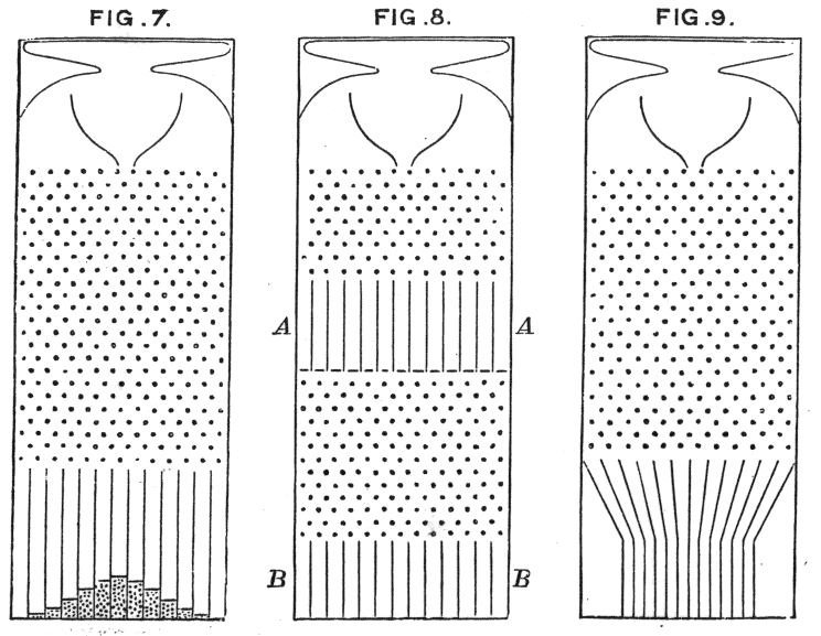
• The name of the language comes from a physical device for visualizing probability distributions because that’s what it does.

---

I will likely do a whole series on Bean Machine later on this autumn, but for today let me just give you the brief overview should you not want to go through the paper. As the paper’s title says, Bean Machine is a Probabilistic Programming Language (PPL).

For a detailed introduction to PPLs you should read my “Fixing Random” series, where I show how we could greatly improve support for analysis of randomness in .NET by both adding types to the base class library and by adding language features to a language like C#.

If you don’t want to read that 40+ post introduction, here’s the TLDR.

We are all used to two basic kinds of programming: produce an effect and compute a result. The important thing to understand is that Bean Machine is firmly in the “compute a result” camp. In our PPL the goal of the programmer is to declaratively describe a model of how the world works, then input some observations of the real world in the context of the model, and have the program produce posterior distributions of what the real world is probably like, given those observations. It is a language for writing statistical model simulations.

A “hello world” example will probably help. Let’s revisit a scenario I first discussed in part 30 of Fixing Random: flipping a coin that comes from an unfair mint. That is, when you flip a coin from this mint, you do not necessarily have a 50-50 chance of getting heads vs tails. However, we do know that when we mint a coin, the distribution of fairness looks like this:

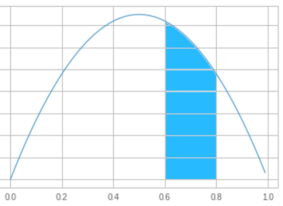
Fairness is along the x axis; 0.0 means “always tails”, 1.0 means “always heads”. The probability of getting a coin of a particular fairness is proportional to the area under the graph. In the graph above I highlighted the area between 0.6 and 0.8; the blue area is about 25% of the total area under the curve, so we have a 25% chance that a coin will be between 0.6 and 0.8 fair.

Similarly, the area between 0.4 and 0.6 is about 30% of the total area, so we have a 30% chance of getting a coin whose fairness is between 0.4 and 0.6. You see how this goes I’m sure.

Suppose we mint a coin; we do not know its true fairness, just the distribution of fairness above. We flip the coin 100 times, and we get 72 heads, 28 tails. What is the most probable fairness of the coin?

Well, obviously the most probable fairness of a coin that comes up heads 72 times out of 100 is 0.72, right?

Well, no, not necessarily right. Why? Because the prior probability that we got a coin that is between 0.0 and 0.6 is rather a lot higher than the prior probability that we got a coin between 0.6 and 1.0. It is possible by sheer luck to get 72 heads out of 100 with a coin between 0.0 and 0.6 fairness, and those coins are more likely overall.

---

Aside: If that is not clear, try thinking about an easier problem that I discussed in my earlier series. You have 999 fair coins and one double-headed coin. You pick a coin at random, flip it ten times and get ten heads in a row. What is the most likely fairness, 0.5 or 1.0? Put another way: what is the probability that you got the double-headed coin? Obviously it is not 0.1%, the prior, but nor is it 100%; you could have gotten ten heads in a row just by luck with a fair coin. What is the true posterior probability of having chosen the double-headed coin given these observations?

---

What we have to do here is balance between two competing facts. First, the fact that we’ve observed some coin flips that are most consistent with 0.72 fairness, and second, the fact that the coin could easily have a smaller (or larger!) fairness and we just got 72 heads by luck. The math to do that balancing act to work out the true distribution of possible fairness is by no means obvious.

What we want to do is use a PPL like Bean Machine to answer this question for us, so let’s build a model!

The code will probably look very familiar, and that’s because Bean Machine is a declarative language based on Python; all Bean Machine programs are also legal Python programs. We begin by saying what our “random variables” are.

---

Aside: Statisticians use “variable” in a way very different than computer programmers, so do not be fooled here by your intuition. By “random variable” we mean that we have a distribution of possible random values; a representation of any single one of those values drawn from a distribution is a “random variable”. 

---

To represent random variables we declare a function that returns a pytorch distribution object for the distribution from which the random variable has been drawn. The curve above is represented by the function beta(2, 2), and we have a constructor for an object that represents that distribution in the pytorch library that we’re using, so:

@random_variable
def coin():
  return Beta(2.0, 2.0)

Easy as that. Every usage in the program of coin() is logically a single random variable; that random variable is a coin fairness that was generated by sampling it from the beta(2, 2) distribution graphed above.

---

Aside: The code might seem a little weird, but remember we do these sorts of shenanigans all the time in C#. In C# we might have a method that looks like it returns an int, but the return type is Task<int>; we might have a method that yield returns a double, but the return type is IEnumerable<double>. This is very similar; the method looks like it is returning a distribution of fairnesses, but logically we treat it like a specific fairness drawn from that distribution.

---

What do we then do? We flip a coin 100 times. We therefore need a random variable for each of those coin flips:

@random_variable
def flip(i):
  return Bernoulli(coin())

Let’s break that down. Each call flip(0), flip(1), and so on on, are distinct random variables; they are outcomes of a Bernoulli process — the “flip a coin” process — where the fairness of the coin is given by the single random variable coin(). But every call to flip(0) is logically the same specific coin flip, no matter how many times it appears in the program.

For the purposes of this exercise I generated a coin and simulated 100 coin tosses to simulate our observations of the real world. I got 72 heads. Because I can peek behind the curtain for the purposes of this test, I can tell you that the coin’s true fairness was 0.75, but of course in a real-world scenario we would not know that. (And of course it is perfectly plausible to get 72 heads on 100 coin flips with a 0.75 fair coin.)

We need to say what our observations are.  The Bernoulli distribution in pytorch produces a 1.0 tensor for “heads” and a 0.0 tensor for “tails”. Our observations are represented as a dictionary mapping from random variables to observed values.

heads = tensor(1.0)
tails = tensor(0.0)
observations = {
  flip(0) : heads,
  flip(1) : tails,
  ...  and so on, 100 times with 72 heads, 28 tails.
}

Finally, we have to tell Bean Machine what to infer. We want to know the posterior probability of fairness of the coin, so we make a list of the random variables we care to infer posteriors on; there is only one in this case.

inferences = [ coin() ]
posteriors = infer(observations, inferences)
fairness = posteriors[coin()]

and we get an object representing samples from the posterior fairness of the coin given these observations. (I’ve simplified the call site to the inference method slightly here for clarity; it takes more arguments to control the details of the inference process.)

The “fairness” object that is handed back is the result of efficiently simulating the possible worlds that get you to the observed heads and tails; we then have methods that allow you to graph the results of those simulations using standard graphing packages:

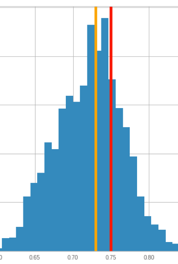
The orange marker is our original guess of observed fairness: 0.72. The red marker is the actual fairness of the coin used to generate the observations, 0.75. The blue histogram shows the results of 1000 simulations; the vast majority of simulations that produced those 72 heads had a fairness between 0.6 and 0.8, even though only 25% of the coins produced by the mint are in that range.  As we would hope, both the orange and red markers are near the peak of the histogram.

So yes, 0.72 is close to the most likely fairness, but we also see here that a great many other fairnesses are possible, and moreover, we clearly see how likely they are compared to 0.72. For example, 0.65 is also pretty likely, and it is much more likely than, say, 0.85. This should make sense, since the prior distribution was that fairnesses closer to 0.5 are more likely than those farther away; there’s more “bulk” to the histogram to the left than the right: that is the influence of the prior on the posterior!

Of course because we only did 1000 simulations there is some noise; if we did more simulations we would get a smoother result and a clear, single peak. But this is a pretty good estimate for a Python program with six lines of model code that only takes a few seconds to run.

---

Why do we care about coin flips? Obviously we don’t care about solving coin flip problems for their own sake. Rather, there are a huge number of real-world problems that can be modeled as coin flips where the “mint” produces unfair coins and we know the distribution of coins that come from that mint:

• A factory produces routers that have some “reliability”; each packet that passes through each router in a network “flips a coin” with that reliability; heads, the packet gets delivered correctly, tails it does not. Given some observations from a real data center, which is the router that is most likely to be the broken one? I described this model in my Fixing Random series.
• A human reviewer classifies photos as either “a funny cat picture” or “not a funny cat picture”. We have a source of photos — our “mint” — that produces pictures with some probability of them being a funny cat photo, and we have human reviewers each with some individual probability of making a mistake in classification. Given a photo and ten classifications from ten reviewers, what is the probability that it is a funny cat photo? Again, each of these actions can be modeled as a coin flip.
• A new user is either a real person or a hostile robot, with some probability. The new user sends a friend request to you; you either accept it or reject it based on your personal likelihood of accepting friend requests. Each one of these actions can be modeled as a coin flip; given some observations of all those “flips”, what is the posterior probability that the account is a hostile robot?

And so on; there are a huge number of real-world problems we can solve just with modeling coin flips, and Bean Machine does a lot more than just coin flip models!

---

I know that was rather a lot to absorb, but it is not every day you get a whole new programming language to explain! In future episodes I’ll talk more about how Bean Machine works behind the scenes, how we traded off between declarative and imperative style, and that sort of thing. It’s been a fascinating journey so far and I can’t hardly wait to share it.