[Code is here.]

Last time on FAIC we discovered the interesting fact that conditional probabilities can be represented as likelihood functions, and that applying a conditional probability to a prior probability looks suspiciously like SelectMany, which is usually the bind operation on the sequence monad. We created a new implementation of SelectManythat creates an object which samples from the prior, calls the likelihood, and then samples from the resulting distribution. Is that the bind operation on the probability distribution monad?

Aside: If you’re completely confused by the preceding paragraph, you might want to read my gentle introduction to monads for OO programmers. Go ahead and read that over if it is not fresh in your mind.

We need the following things to have a monad in C#:

• We need an “embarrassingly generic” type: some Foo<T> where it can sensibly take on any T whatsoever. IDiscreteDistribution<T> meets that condition.
• The type represents an “amplification of power” of the underlying type. Indeed it does; it allows us to represent a probability distribution of particular values of that type, which is certainly a new power that we did not have before.
• We need a way of taking any specific value of any T, and creating an instance of the monadic type that represents that specific value. Singleton.Distribution(t) meets that condition.
• There is frequently(but not necessarily) an operation that extracts a value of the underlying type from an instance of the monad. Sample() is that operation. Note that sampling a singleton always gives you back the original value.
• There is a way to “bind” a new function onto an existing instance of the monad. That operation has the signature M<R> SelectMany<A, R>(M<A> m, Func<A, M<R>> f).  We traditionally call it SelectMany in C# because that’s the bind operation on IEnumerable<T>, and it produces a projection on all the elements from a sequence of sequences. As we saw last time, we have this function for probability distributions.
• Binding the “create a new instance” function to an existing monad must produce an equivalent monad. I think it is pretty clear that if we have an IDiscreteDistribution in hand, call it d, that SelectMany(d, t => Singleton.Distribution(t)) produces an object that has the same distribution that d does. If that’s not clear, play around with the code until it becomes clear to you.
• Going “the other direction” must also work. That is, if we have a Func<A, IDiscreteDistribution<B>> called f, and a value of A, then SelectMany(Singleton<A>.Distribution(a), f) and f(a) must produce logically the same IDiscreteDistribution<B>. Again, if that’s not clearly true in your mind, step through the code mentally or write some sample code and convince yourself that it is true.
• Two bind operations “on top of each other” must produce the same logical result as a single bind that is the composition of the two bound functions. That’s maybe a little vague; see Part 7 of my series on monads for details. Suffice to say, we meet this condition as well.

All our conditions are met; IDiscreteDistribution<T> is a monad. So we should be able to use it in a query comprehension, right?

from c in cold
from s in SneezedGivenCold(c)
select s

Unfortunately this gives an error saying that SelectMany cannot be found; what’s up with that?

The query comprehension syntax actually requires a slight variation on the traditional “bind” operation; it requires that we also allow a projection on the end, and that moreover, the projection take both the original value and the transformed value. That is, C# requires us to implement it like this:

public sealed class Combined<A, B, C> :
  IDiscreteDistribution<C>
{
  private readonly List<C> support;
  private readonly IDiscreteDistribution<A> prior;
  private readonly Func<A, IDiscreteDistribution<B>> likelihood;
  private readonly Func<A, B, C> projection;
  public static IDiscreteDistribution<C> Distribution(
      IDiscreteDistribution<A> prior, 
      Func<A, IDiscreteDistribution<B>> likelihood, 
      Func<A, B, C> projection) =>
    new Combined<A, B, C>(prior, likelihood, projection);
  private Combined(
    IDiscreteDistribution<A> prior, 
    Func<A, IDiscreteDistribution<B>> likelihood, 
    Func<A, B, C> projection)
  {
    this.prior = prior;
    this.likelihood = likelihood;
    this.projection = projection;
    var s = from a in prior.Support()
            from b in this.likelihood(a).Support()
            select projection(a, b);
            this.support = s.Distinct().ToList();
  }
  public IEnumerable<C> Support() =>
     this.support.Select(x => x);
  public int Weight(C c) => NOT YET!
  public C Sample()
  {
    A a = this.prior.Sample();
    B b = this.likelihood(a).Sample();
    return this.projection(a, b);
  }
}

And now we can implement SelectMany as

public static IDiscreteDistribution<C> SelectMany<A, B, C>(
    this IDiscreteDistribution<A> prior,
    Func<A, IDiscreteDistribution<B>> likelihood,
    Func<A, B, C> projection) =>
  Combined<A, B, C>.Distribution(prior, likelihood, projection);

and of course if we want a SelectMany with the traditional monad bind signature, that’s just

public static IDiscreteDistribution<B> SelectMany<A, B>(
    this IDiscreteDistribution<A> prior,
    Func<A, IDiscreteDistribution<B>> likelihood) =>
  SelectMany(prior, likelihood, (a, b) => b);

Now that we have aSelectMany, we can write conditional probabilities in comprehension syntax, as before:

var sneezed = from c in cold
              from s in SneezedGivenCold(c)
              select s;

or, if we like, we can extract a tuple giving us both values:

public static IDiscreteDistribution<(A, B)> Joint<A, B>(
    this IDiscreteDistribution<A> prior,
    Func<A, IDiscreteDistribution<B>> likelihood) =>
  SelectMany(prior, likelihood, (a, b) => (a, b));

var joint = cold.Joint(SneezedGivenCold);

and if we graph that, we see that we get the distribution we worked out by hand from last episode:

Console.WriteLine(sneezed.Histogram());
Console.WriteLine(sneezed.ShowWeights());
Console.WriteLine(joint.Histogram());
Console.WriteLine(joint.ShowWeights());

 No|****************************************
Yes|*****
 No:111
Yes:14

  (No, No)|****************************************
 (No, Yes)|*
 (Yes, No)|
(Yes, Yes)|***
  (No, No):873
 (No, Yes):27
 (Yes, No):15
(Yes, Yes):85

Aside: Of course I am cheating slightly here because I have not yet implemented the weight function on the combined distribution; we’ll get to that next time!

It might seem slightly vexing that C# requires us to implement a variation on the standard bind operation, but in this case it is actually exactly what we want. Why’s that?

Let’s remind ourselves of how we are notating probability distributions. If we have a collection of possible outcomes of type Cold, we notate that distribution as P(Cold); since Cold has two possibilities, this distribution is made up from two probabilities, P(Cold.Yes) and P(Cold.No) which add up to 100%. We represent this in our type system as IDiscreteDistribution<Cold>

A conditional probability distribution P(Sneezed|Cold) is “given a value from type Cold, what is the associated distribution P(Sneezed)“?  In other words, it is Func<Cold, IDiscreteDistribution<Sneezed>>.

What then is P(Cold&Sneezed)?  That is our notation for the joint distribution over all possible pairs. This is made up of four possibilities: P(Cold.No & Sneezed.No), P(Cold.No&Sneezed.Yes), P(Cold.Yes&Sneezed.No), and P(Cold.Yes&Sneezed.Yes), which also add up to 100%.

In our type system, this is IDiscreteDistribution<(Cold, Sneezed)>

Now, remember the fundamental law of conditional probability is:

P(A) P(B|A) = P(A&B)

That is, the probability of A and B both occurring is the probability of A occurring, multiplied by the probability of B occurring given that A has.

That is, we can pick any values from those types, say:

P(Cold.Yes) P(Sneezed.Yes|Cold.Yes) = P(Cold.Yes&Sneezed.Yes)

That is, the probability of some value of A and some value of B both occurring is the probability of the value of A occurring multiplied by the probability of the value of B given that the value of A has occurred.

Aside: “multiplication” here is assuming that the probabilities are between 0.0 and 1.0, but again, squint a little and you’ll see that it’s all just weights. In the next episode we’ll see how to compute the weights as integers by thinking about how to do the multiplication in fractions.

We’ve implemented P(A) as IDiscreteDistribution<A>, we’ve implemented P(B|A) as Func<A, IDiscreteDistribution<B>>, and P(A&B) as IDiscreteDistribution<(A, B)>.

We have a function Joint<A, B>​ that takes the first two and gives you the third, and if you work out the math, you’ll see that the probabilities of each member of the joint distribution that results are the products of the probabilities given from the prior and the likelihood. Multiplication of a prior probability by a likelihood across all members of a type is implemented by SelectMany. 

Coming up on FAIC: We’ll work out the weights correctly, and that will enable us to build an optimized  SelectMany implementation.

[Code is here.]

Last time on FAIC we implemented an efficient “conditioned” probability using the Where operator on distributions; that is, we have some “underlying” distribution, and we ask the question “if a particular condition has to be met, what is the derived distribution that meets that condition?” For discrete distributions we can compute that distribution directly and just return it.

There is another kind of conditional probability though, which is much more rich, complex and counter-intuitive, and that is exploring the relationship between “what is the probability of X?” and “what is the probability of Y given that we know X?”

For example: pick a random person in the world who has a cold. What is the probability that they sneezed in the last 24 hours? Probably something like 85%.

Now pick a random person who does not have a cold. For them, the probability is maybe more like 3%. In months when I do not have a cold, I sneeze maybe one or two days.

So what we’ve got here is a rather more complex probability distribution; in fact we have two entirely different distributions, and which one we use depends on a condition.

Notice how this is clearly related to our recent discussion of conditioned probabilities, but different. With a “Where” clause we are saying make the support of this distribution smaller because some outcomes are impossible based on a condition. What we’re talking about here is choosing between two (or more) distributions depending on a condition.

The standard notation for this kind of probability in mathematics is a bit unfortunate. We would say something like P(sneezed|no cold ) = 0.03 to represent “3% chance that I sneezed if I didn’t have a cold” and P(sneezed|cold) = 0.85 to represent “85% chance that I sneezed if I had a cold”. That is, the syntax is P(A|B) means “what is the probability of A given that B happened?”

How might we represent this in our system? It seems like IDiscreteDistribution<T> is not rich enough. Let’s just start making some types and see what we can come up with.

“Has sneezed recently” and “has a cold” are Booleans, but I want the types of everything to be very clear in the analysis which follows, so I’m going to make my own custom types:

enum Cold { No, Yes }
enum Sneezed { No, Yes }

I want to be slightly abusive of notation here and say that P(Cold.Yes) and P(Cold.No) are the weights of a probability distribution that I’m going to call by the shorthand P(Cold). Similarly for P(Sneezed); that’s the probability distribution that gives weights to P(Sneezed.Yes) and P(Sneezed.No). Normally we think of P(something) as being a value between 0.0 and 1.0, but if you squint at it, really those values are just weights. It doesn’t matter what convention we use for weights; a bunch of integers that give ratios of probabilities and a bunch of doubles that give fractions have pretty much the same information content.

Plainly what I would very much like is to have IDiscreteDistribution<Cold> be the C# type that represents P(Cold).

But how can we represent our concept of “There’s a 3% chance I sneezed if I do not have a cold, but an 85% chance if I do have a cold?”

That sure sounds like precisely this:

IDiscreteDistribution<Sneezed> SneezedGivenCold(Cold c)
{
  var list = new List<Sneezed>() { Sneezed.No, Sneezed.Yes };
  return c == Cold.No ?
    list.ToWeighted(97, 3) :
    list.ToWeighted(15, 85);
}

That is, if we do not have a cold then the odds are 97 to 3 that we did not sneeze, and if we do have a cold, then the odds is 15 to 85 that we did not sneeze.

I’ve said that I want to represent P(Cold.Yes) and P(Cold.No) by the shorthand P(Cold), and that plainly this in our type system is IDiscreteDistribution<Cold>. Now I want to represent the notion of P(Sneezed) given a value of Cold as P(Sneezed|Cold), which is implemented by the function above. So, what type in our type system is that? Well, suppose we wanted to assign SneezedGivenCold to a variable; what would its type be? Clearly the type of P(Sneezed|Cold) is Func<Cold, IDiscreteDistribution<Sneezed>>!

How interesting! Conditional probabilities are actually functions.

This sort of function has a name; it is called a likelihood function. That is, given some condition, how likely is some outcome?

So that’s interesting, but how is this useful?

Let’s randomly choose a person in the world, where we do not know whether they have a cold or not. What is the probability that they sneezed recently? It depends entirely on the prevalence of colds! If 100% of the world has a cold, then there’s an 85% chance that a randomly chosen person sneezed recently, but if 0% of the world has a cold, then there’s only a 3% chance. And if it is somewhere in between, the probability will be different from either 85% or 3%.

To solve this problem we need to know the probability that the person we’ve chosen has a cold. The probability that some randomly chosen person has a cold is called the prior probability.

What if 10% of the world has a cold? Let’s work it out by multiplying the probabilities:

 Cold      Sneezed       Result
 (prior)   (likelihood)  (conditional)
 10% Yes   85% Yes       8.5% have a cold, and sneezed
           15% No        1.5% have a cold, did not sneeze
 90% No     3% Yes       2.7% do not have a cold, and sneezed
           97% No       87.3% do not have a cold, did not sneeze

Sure enough those probabilities in the right column add up to 100%. The probability that a randomly chosen person in the world sneezed recently (given that these numbers that I made up are accurate) is 8.5% + 2.7% = 11.2%.

The rightmost column of the table that I’ve sketched out here is called the joint probability, which we’ll notate as P(Cold&Sneezed).

We can write this table more compactly like this:

             Cold Yes    Cold No   Total
Sneezed Yes     8.5%        2.7%   11.2%
Sneezed No      1.5%       87.3%   88.8%
Total            10%         90%    100%

The rightmost column of this table is called the marginal probability, so-called because of the way the sums end up at the margins of the table.

What if we expressed the marginal probability as integers? The odds that a random person has sneezed is 11.2% to 88.8%, which if you work out the math, is exactly odds of 14 to 111.

Aside: when I was debugging the code to compute the weights that we will see in a future episode, I got “111” printed out when I was primed to see “112”, having just computed “11.2%” by hand. I almost went on a lengthy bug hunt looking for the non-existing off-by-one error. Fortunately I stopped and double-checked my work, and realized that the 111 represents the 88.8%, not the 11.2%.

How can we do this math given the set of types we’ve created so far? Let’s start with the prior:

var colds = new List<Cold>() { Cold.No, Cold.Yes };
IDiscreteDistribution<Cold> cold = colds.ToWeighted(90, 10);

We’ve got the prior, and we’ve got the likelihood function SneezedGivenCold. We would like to get the marginal probability IDiscreteDistribution<Sneezed>​.

We could implement such a distribution by first sampling from the prior, then calling SneezedFromCold, and then sampling from the returned distribution. Let’s implement it.

Aside: We are of course assuming that the likelihood function is pure.

public sealed class Combined<A, R> : IDiscreteDistribution<R>
{
  private readonly List<R> support;
  private readonly IDiscreteDistribution<A> prior;
  private readonly Func<A, IDiscreteDistribution<R>> likelihood;
  public static IDiscreteDistribution<R> Distribution(
      IDiscreteDistribution<A> prior,
      Func<A, IDiscreteDistribution<R>> likelihood) =>
    new Combined<A, R>(prior, likelihood);
  private Combined(
    IDiscreteDistribution<A> prior,
    Func<A, IDiscreteDistribution<R>> likelihood)
  {
    this.prior = prior;
    this.likelihood = likelihood;
    var q = from a in prior.Support()
            from b in this.likelihood(a).Support()
            select b;
    this.support = q.Distinct().ToList();
  }
  public IEnumerable<R> Support() =>
    this.support.Select(x => x);
  public R Sample() =>
    this.likelihood(this.prior.Sample()).Sample();
  public int Weight(R r) => WE’LL COME BACK TO THIS ONE
}

We haven’t implemented Weight, but we don’t need it to run a histogram. Let’s try it out:

Combined<Cold, Sneezed>.Distribution(cold, SneezedGivenCold)
  .Histogram()

 No|****************************************
Yes|****

Sure enough, it looks like there is about an 11% chance that a randomly chosen person sneezed, given these distributions.

Now, of course as I have done throughout this series, let’s make a little helper function to make the call sites look a little nicer:

public static IDiscreteDistribution<R> MakeCombined<A, R>(
    this IDiscreteDistribution<A> prior,
    Func<A, IDiscreteDistribution<R>> likelihood) => 
  Combined<A, R>.Distribution(prior, likelihood);

Once again, that should look very familiar! I should change the name of this helper.

If you are still surprised at this point, you have not been paying attention. I’ve already made Select and Where, so the obvious next step is…

public static IDiscreteDistribution<R> SelectMany<A, R>(
    this IDiscreteDistribution<A> prior,
    Func<A, IDiscreteDistribution<R>> likelihood) => 
  Combined<A, R>.Distribution(prior, likelihood);

… the bind operation on the probability monad.

And the inelegant call site above is now the much more clear:

cold.SelectMany(SneezedGivenCold).Histogram()

Coming up on FAIC: We’ll verify that the distribution type really is a monad, and make a few tweaks to get it working with query comprehension syntax. Then we’ll figure out how to implement the Weight​ function.

[Code is here.]

Last time on FAIC we drew a line in the sand and required that the predicates and projections used by Where and Select on discrete distributions be “pure” functions: they must complete normally, produce no side effects, consume no external state, and never change their behaviour. They must produce the same result when called with the same argument, every time. If we make these restrictions then we can get some big performance wins out of Where and Select. Let’s see how.

The biggest problem we face is that possibly-long-running loop in the Where; basically we are rejection-sampling the distribution, and we know that can take a long time. Is there a way to directly produce a new distribution that can be efficiently sampled?

Of course there is, and it was a little silly of us to miss it. Let’s make a helper method:

public static IDiscreteDistribution<T> ToWeighted<T>(
    this IEnumerable<T> items,
    IEnumerable<int> weights)
{
  var list = items.ToList();
  return WeightedInteger.Distribution(weights)
    .Select(i => list[i]);
}

There’s an additional helper method I’m going to need in a couple of episodes, so let’s just make it now:

public static IDiscreteDistribution<T> ToWeighted<T>(
    this IEnumerable<T> items,
    params int[] weights) =>
items.ToWeighted((IEnumerable<int>)weights);

And now we can delete our Conditioned class altogether, and replace it with:

public static IDiscreteDistribution<T> Where<T>(
  this IDiscreteDistribution<T> d,
  Func<T, bool> predicate)
{
  var s = d.Support().Where(predicate).ToList();
  return s.ToWeighted(s.Select(t => d.Weight(t)));
}

Recall that the WeightedInteger factory will throw if the support is empty, and return a Singleton or Bernoulli if it size one or two; we don’t have to worry about that. No more maybe-long-running loop! We do at most two underlying samples per call to Sample now.

Exercise: We’re doing probabilistic workflows here; it seems strange that we are either 100% rejecting or 100% accepting in Where. Can you write an optimized implementation of this method?

public static IDiscreteDistribution<T> Where<T>(
  this IDiscreteDistribution<T> d,
  Func<T, IDiscreteDistribution<bool>> predicate)

That is, we accept each T with a probability distribution given by a probabilistic predicate.

This one will be easier to implement once we have the gear we’re going to develop a few episodes from now, but I mention it now to get you thinking about the problem.

That takes care of optimizing Where. What about optimizing Select?

Of course we can do the same trick. We just have to take into account the fact that the projection might cause some members of the underlying support to “merge” their weights:

public static IDiscreteDistribution<R> Select<A, R>(
  this IDiscreteDistribution<A> d,
  Func<A, R> projection)
{
  var dict = d.Support()
              .GroupBy(projection, a => d.Weight(a))
              .ToDictionary(g => g.Key, g => g.Sum());
  var rs = dict.Keys.ToList();
  return Projected<int, R>.Distribution(
    WeightedInteger.Distribution(
      rs.Select(r => dict[r])),
      i => rs[i]);
}

That is: we compute the new support, and the weights for each element of it. Now we can construct a weighted integer distribution that chooses an offset into the support.

Exercise: Why did I not write the far more concise:

  return rs.ToWeighted(rs.Select(r => dict[r])));

?

Let’s think for a minute about whether this really does what we want. Suppose for example we do a projection on a Singleton:

• We’ll end up with a single-item dictionary with some non-zero weight.
• The call to the weighted integer factory will return a Singleton<int> that always returns zero.
• We’ll build a projection on top of that, and the projection factory will detect that the support is of size one, and return a Singleton<T> with the projected value.

Though we’ve gone through a bunch of unnecessary object constructions, we end up with what we want.

Furthermore, suppose we have a projection, and we do a Select on that: we avoid the problem we have in LINQ-to-objects, where we build a projection on top of a projection and end up with multiple objects representing the workflow.

Aside: That last sentence is an oversimplification; in LINQ-to-objects there is an optimization for this scenario; we detect Select-on-Select (and Select-on-Where and so on) and build up a single object that represents the combined projection, but that single object still calls all the delegates. So in that sense there are still many objects in the workflow; there’s just a single object coordinating all the delegates.

In this scenario we spend time up front calling the projection on every member of the support once, so we don’t need to ever do it later.

Again, I’m not trying make the series of factories here the most efficient it could be; we’re creating a lot of garbage. Were I building this sort of system for industrial use, I’d be more aggressive about taking early outs that prevent this sort of extra allocation. What I’m trying to illustrate here is that we can use the rules of probability (and the fact that we have pure predicates and projections) to produce distribution objects that give the correct results.

Aside: Of course, none of this fixes the original problems with weighted integer: that in the original constructor, we do not optimize away “all weights zero except one” or “trailing zeros”. Those improvements are still left as exercises.

Next time on FAIC: we’ve seen that we can use Where​ to filter a distribution to make a conditioned distribution; we’ll look at a more rich and complex way to represent conditional probabilities, and discover a not-so-surprising fact about our distribution interface.

[Code is here.]

We’re going to spend the next while in this series on expressing probabilities that have some sort of extra condition associated with them. We’ll start with a simple example: I want to roll a fair six-sided die, but discard the threes. Why? Maybe I really dislike threes. Doesn’t matter; we will want to be able to create new distributions by putting conditions on other distributions, so let’s figure out how to do so.

Now, of course, we could create the desired distribution easily enough; as we know from last time on FAIC, it is

WeightedInteger.Distribution(0, 1, 1, 0, 1, 1, 1)

But suppose we have a distribution already in hand which we wish to apply a condition to, post hoc. I’m not going to labour the point; we can see how to do that easily enough. It’s a variation on our “projected” distribution from a while back:

public sealed class Conditioned<T> :
  IDiscreteDistribution<T>
{
  private readonly List<T> support;
  private readonly IDiscreteDistribution<T> underlying;
  private readonly Func<T, bool> predicate;
  public static IDiscreteDistribution<T> Distribution(
    IDiscreteDistribution<T> underlying,
    Func<T, bool> predicate)
  {
    var d = new Conditioned<T>(underlying, predicate);
    if (d.support.Count == 0)
      throw new ArgumentException();
    if (d.support.Count == 1)
      return Singleton<T>.Distribution(d.support[0]);
    return d;
  }
  private Conditioned(
    IDiscreteDistribution<T> underlying,
    Func<T, bool> predicate)
  {
    this.underlying = underlying;
    this.predicate = predicate;
    this.support = underlying.Support()
      .Where(predicate)
      .ToList();
  }
  public T Sample()
  {
    while (true) // Ouch
    {
      T t = this.underlying.Sample();
      if (this.predicate(t))
          return t;
    }
  }
  public IEnumerable<T> Support() =>
    this.support.Select(x => x);
  public int Weight(T t) =>
    predicate(t) ? underlying.Weight(t) : 0;
}

Given our discussion a few episodes back about projected distributions and the fact that creating them has the same signature as “Select”, I’m sure it will come as no surprise to you that I’m going to make a helper method:

public static IDiscreteDistribution<T> Where<T>(
    this IDiscreteDistribution<T> d,
    Func<T, bool> predicate) =>
  Conditioned<T>.Distribution(d, predicate);

And you know what this means: I get to use comprehension syntax again!

var noThrees = from roll in SDU.Distribution(1, 6)
               where roll != 3
               select roll;
Console.WriteLine(noThrees.Histogram());

And we get as expected, no threes:

1|***************************************
2|***************************************
4|***************************************
5|***************************************
6|***************************************

However, there are some problems here. That possibly-long-running loop is deeply worrisome. In fact, dealing with the existence of that loop will be the major theme of the rest of this series, in one way or another. (This should feel familiar; of course this is just another version of the “rejection sampling” problem from a few episodes ago.)

We’ll talk about that loop problem more in the next episode. For the remainder of this episode I want to examine an assumption I made in the code above; it’s the same assumption that I made when we discussed projections. We just blew right past it, but this assumption introduces what might be characterized as a serious bug.

Consider the following code, which uses only sequences, no distributions:

int filterOut = 3;
Func<int, bool> predicate = x => x != filterOut;
var range = Enumerable.Range(1, 6).Where(predicate);
Console.WriteLine(range.CommaSeparated());
filterOut = 4;
Console.WriteLine(range.CommaSeparated());

Aside: I got sick of typing string.Join(… blah blah blah…) so I made a handful of extension methods to be a little more fluent. See the source code for details.)

If you recall that sequences are computed lazily and lambdas are closed over variables, not values, then this output should be expected:

1,2,4,5,6
1,2,3,5,6

What if we do the same thing to distributions?

int filterOut = 3;
Func<int, bool> predicate = x => x != filterOut;
var d = SDU.Distribution(1, 6).Where(predicate);
Console.WriteLine(d.Samples().Take(10).CommaSeparated());
filterOut = 4;
Console.WriteLine(d.Samples().Take(10).CommaSeparated());

As we’d expect, we first get no threes, and then no fours:

1,1,4,6,6,5,4,1,2,6
6,5,6,5,1,5,6,3,2,1

So what’s the problem?

Console.WriteLine(d.Support().CommaSeparated());

1,2,4,5,6

Uh oh. We just produced a 3 in a distribution that does not list 3 in its support!

Why? Because I computed the support in the constructor and cached it, but the support changed when the predicate changed its behaviour, and it is now out-of-date. The object is now lying to us.

Obviously I could fix this problem easily enough: do not compute the support in the constructor; compute it dynamically, on demand. Is that the right thing to do?

If we do, we lose the ability to reject “null” distributions — distributions with no support — and therefore it is possible to get into a situation where sampling hangs because the predicate is never true. (We could re-check the support before every sample, and throw if the support is empty, but that seems expensive.)

Furthermore, as we’ll see in the next few episodes, we can do some pretty good optimizations if we can assume that the predicate does not change.

I’m therefore going to state right now that the predicate passed to Where (and the projection passed to Select) must be “pure” functions when they are intended to operate on probability distributions.

A “pure” function for our purposes has the following characteristics:

• It must complete normally; in its regular operation it should not hang and it should not throw. It is permissible for a pure function to throw if its preconditions are violated; for example, a pure function that is documented as not taking negative numbers is permitted to throw an argument exception if passed a negative number. But a pure function should not throw or hang when given a normal, expected input.
• It must not produce any side effect. For example, it must not write to the console or mutate a global variable or anything like that.
• Its outputs must depend solely on its inputs; a pure method does not produce one result on its first call and a different result on its second call because something in the world changed; the only reason to produce a different result is if the arguments passed in are different.

Pure functions are nice to work with in two particular ways. First, you can reason about their correctness entirely “locally”; you do not have to consider the state of the world at the time the call is made, and you do not have to worry that the state of the world will change depending on how many times the call happens. Second, you can get performance wins by taking advantage of the fact that you know that two calls with the same arguments will produce the same result.

Unfortunately, in C# we have no good way of detecting a non-pure method at compile time and outlawing them as arguments to Where and Select; we will have to rely on the user being smart enough to not shoot themselves in the foot here.

Next time on FAIC: Now that we are requiring purity in Where and Select, what optimizations can we make to the discrete distributions we’ve created so far?

[Code is here.]

Last time on FAIC I sketched out the “alias method”, which enables us to implement sampling from a weighted discrete distribution in constant time. The implementation is slightly tricky, but we’ll go through it carefully.

The idea here is:

• If we have n weights then we’re going to make n distributions.
• Every distribution is either a singleton that returns a particular number, or we use a projection on a Bernoulli to choose between two numbers.
• To sample, we uniformly choose from our n distributions, and then we sample from that distribution, so each call to Sample on the weighted integer distribution does exactly two samples of other, simpler distributions.

How are we going to implement it? The key insight is: weights which are lower than the average weight “borrow” from weights which are higher than average.

Call the sum of all weights s. We start by multiplying each weight by n, which gives us s * n “weight points” to allocate; each of the n individual distributions will have a total weight of s points.

private readonly IDistribution<int>[] distributions;
private WeightedInteger(IEnumerable<int> weights)
{
  this.weights = weights.ToList();
  int s = this.weights.Sum();
  int n = this.weights.Count;
  this.distributions = new IDistribution<int>[n];

All right, I am going to keep track of two sets of “weight points”: elements where the unallocated “weight points” are lower than s, and elements where it is higher than s. If we’ve got a weight that is exactly equal to the average weight then we can just make a singleton.

  var lows = new Dictionary<int, int>();
  var highs = new Dictionary<int, int>();
  for(int i = 0; i < n; i += 1)
  {
    int w = this.weights[i] * n;
    if (w == s)
      this.distributions[i] = Singleton<int>.Distribution(i);
    else if (w < s)
      lows.Add(i, w);
    else
      highs.Add(i, w);
  }

If every element’s weight was average, then we’re done; the dictionaries are empty. (And we should not have created a weighted integer distribution in the first place!)

If not, then some of them must have been above average and some of them must have been below average. This isn’t Lake Wobegon; not everyone is above average. Therefore iff we have more work to do then there must be at least one entry in both dictionaries.

What we’re going to do is choose (based on no criteria whatsoever) one “low” and one “high”, and we’re going to transfer points from the high to the low. We’ll start by grabbing the relevant key-value pairs and removing them from their respective dictionaries.

  while(lows.Any())
  {
    var low = lows.First();
    lows.Remove(low.Key);
    var high = highs.First();
    highs.Remove(high.Key);

The high has more than s points, and the low has less than s points; even if the low has zero points, the most we will transfer out of the high is s, so the high will still have some points when we’re done. The low will be full up, and we can make a distribution for it:

    int lowNeeds = s – low.Value;
    this.distributions[low.Key] =
        Bernoulli.Distribution(low.Value, lowNeeds)
          .Select(x => x == 0 ? low.Key : high.Key);

Even if the low column value is zero, we’re fine; Bernoulli.Distribution will return a Singleton. That’s exactly what we want; there is zero chance of getting the low column number.

If the low is not zero-weighted, then we want the low-to-high odds to be in the ratio of the low points to the stolen high points, such that their sum is s; remember, we have n*s points to distribute, and each row must get s of them.

We just filled in the distribution for the “low” element. However, the “high” element still has points, remember. There are three possible situations:

1. the high element has exactly s points remaining, in which case it can become a singleton distribution
2. the high element has more than s points, so we can put it back in the high dictionary
3. the high element has one or more points, but fewer than s points, so it goes in the low dictionary

    int newHigh = high.Value – lowNeeds;
    if (newHigh == s)
      this.distributions[high.Key] =
        Singleton<int>.Distribution(high.Key);
    else if (newHigh < s)
      lows[high.Key] = newHigh;
    else
      highs[high.Key] = newHigh;
  }
}

And we’re done.

• Every time through the loop we remove one element from both dictionaries, and then we add back either zero or one elements, so our net progress is either one or two distributions per iteration.
• Every time through the loop we account for either s or 2s points and they are removed from their dictionaries, and we maintain the invariant that the low dictionary is all the elements with fewer than s points, and the high dictionary is all those with more.
• Therefore we will never be in a situation where there are lows left but no highs, or vice versa; they’ll run out at the same time.

We’ve spent O(n) time (and space) computing the distributions; we can now spend O(1) time sampling. First we uniformly choose a distribution, and then we sample from it, so we have a grand total of two samples, and both are cheap.

public int Sample() 
{
  int i = SDU.Distribution(0, weights.Count – 1).Sample();
  return distributions[i].Sample();
}

Aside: I’ve just committed the sin I mentioned a few episodes ago, of sampling from an array by emphasizing the mechanism in the code rather than building a distribution. Of course we could have made a “meta distribution”  in the constructor with distributions.ToUniform() and then this code would be the delightful

public int Sample() => this.meta.Sample().Sample();

What do you think? is it better in this case to emphasize the mechanism, since we’re in mechanism code, or do the double-sample?

We’ll see in a later episode another elegant way to represent this double-sampling operation, so stay tuned.

Let’s try an example with zeros:

WeightedInteger.Distribution(10, 0, 0, 11, 5).Histogram()

Sure enough:

0|************************************
3|****************************************
4|******************

The alias method is easy to implement and cheap to execute; I quite like it.

Remember, the whole point of this thing is to stop messing around with System.Random when you need randomness. We can now take any set of integer weights and produce a random distribution that conforms to those weights; this is really useful in games, simulations, and so on.

Exercise:  I mentioned a long time ago that I wanted to do all my weights in integers rather than doubles. It is certainly possible to make a weighted integer distribution where the weights are doubles; doing so is left as an exercise.

Be warned: this is a slightly tricky exercise. You have to be very careful when implementing the alias method in doubles because the algorithm I gave depends for its correctness on two properties: (1) every time through the loop, there are exactly s or 2s points removed from the total in the dictionaries, and (2) we are never in a situation where the “high” dictionary still has elements but the “low” dictionary does not, or vice versa.

Those conditions are easily seen to be met when all the quantities involved are small integers. Both those conditions are easily violated because of rounding errors when using doubles, so be extremely careful if you try to implement this using doubles.

Coming up on FAIC: there are (at least) two ways to apply “conditional” probabilistic reasoning; we’ll explore both of them.

[Code is here.]

Last time on FAIC we sketched out an O(log n) algorithm for sampling from a weighted distribution of integers by implementing a discrete variation on the “inverse transform” method where the “inverse” step involves a binary search.

Can we do better than O(log n)? Yes — but we’ll need an entirely different method. I’ll sketch out two methods, and implement one this time, and the other in the next exciting episode.

Again, let’s suppose we have some weights, say 10, 11, 5. We have three possible results, and the highest weight is 11. Let’s construct a 3 by 11 rectangle that looks like our ideal histogram; I’ll put dashes in to more clearly indicate the “spaces”:

0|**********-
1|***********
2|*****------

Here’s an algorithm for sampling from this distribution:

• Uniformly choose a random row and column in the rectangle; it’s easy to choose a number from 0 to 2 for the row and a number from 0 to 10 for the column.
• If that point is a *, then the sample is the generated row number.
• If the point is a –, try again.

Basically, we’re throwing darts at the rectangle, and the likelihood of hitting a valid point on particular row is proportional to the probability of that row.

In case that’s not clear, let’s work out the probabilities. To throw our dart, first we’ll pick a row, uniformly, and then we’ll pick a point in that row, uniformly. We have a 1/3 * 10/11 = 10/33 chance of hitting a star from row 0, an  1/3 * 11/11 = 11/33 chance of hitting a star from row 1, a 1/3 * 5/11 = 5/33 chance of hitting a star from row 2, and that leaves a 7/33 chance of going again. We will eventually pick a *, and the values generated will conform to the desired distribution.

Let’s implement it. We’ll throw away our previous attempt and start over. (No pun intended.)

private readonly List<IDistribution<int>> distributions;
private WeightedInteger(List<int> weights)
{
  this.weights = weights;
  this.distributions =
    new List<IDistribution<int>>(weights.Count);
  int max = weights.Max();
  foreach(int w in weights)
    distributions.Add(Bernoulli.Distribution(w, max – w));
}

All right, we have three distributions; in each, a zero is success and a one is failure. In our example of weights 10, 11, 5, the first distribution is “10 to 1 odds of success”, the second is “always success”, and the third is “5 to 6 odds of success”. And now we sample in a loop until we succeed. We uniformly choose a distribution, and then sample from that distribution until we get success.

public int Sample() 
{
  var rows = SDU.Distribution(0, weights.Count – 1);
  while (true)
  {
    int row = rows.Sample();
    if (distributions[row].Sample() == 0)
      return row;
  }
}

We do two samples per loop iteration; how many iterations are we likely to do? In our example we’ll get a result on the first iteration 26/33 of the time, because we have 26 hits out of 33 possibilities. That’s 79% of the time. We get a result after one or two iterations 95% of the time. The vast majority of the time we are going to get a result in just a handful of iterations.

But now let’s think again about pathological cases. Remember our distribution from last time that had 1000 weights: 1, 1, 1, 1, …, 1, 1001. Consider what that histogram looks like.

   0|*------...---  (1 star, 1000 dashes)
   1|*------...---  (1 star, 1000 dashes)
    [...]
 998|*------...---  (1 star, 1000 dashes)
 999|*******...***  (1001 stars, 0 dashes)

Our first example has 26 stars and 6 dashes. In our pathological example there will be 2000 stars and 999000 dashes, so the probability of exiting the loop on any particular iteration is about one in 500. We are typically going to loop hundreds of times in this scenario! This is far worse than our O(log n) option in pathological cases.

This algorithm is called “rejection sampling” (because we “reject” the samples that do not hit a *) and it works very well if all the weights are close to the maximum weight, but it works extremely poorly if there is a small number of high-weight outputs and a large number of low-weight outputs.

Fortunately there is a way to fix that problem. I’m going to reject rejection sampling, and move on to our third and final technique.

Let’s re-draw our original histogram, but I’m going to make two changes. First, instead of stars I’m going to fill in the number sampled, and I’m going to make it a 33 by 3 rectangle, and triple the size of every row.

0|000000000000000000000000000000---
1|111111111111111111111111111111111
2|222222222222222------------------

Plainly this is logically no different; we could “throw a dart”, and the number that we hit is the sample; if we hit a dash, we go again. But we still have the problem that 21 out of 99 times we’re going to hit a dash.

My goal is to get rid of all the dashes, but I’m going to start by trying to get 7 dashes in each row. There are 21 dashes available, three rows, so that’s seven in each row.

To achieve that, I’m going to first pick an “excessive” row (too many numbers, too few dashes) and “deficient row” (too few numbers, too many dashes) and move some of the numbers from the excessive row to the deficient row, such that the deficient row now has exactly seven dashes. For example, I’ll move eleven of the 0s into the 2 row, and swap eleven of the 2 row’s dashes into the 0 row.

0|0000000000000000000--------------
1|111111111111111111111111111111111
2|22222222222222200000000000-------

We’ve achieved our goal for the 2 row. Now we do the same thing again. I’m going to move seven of the 1s into the 0 row:

0|00000000000000000001111111-------
1|11111111111111111111111111-------
2|22222222222222200000000000-------

We’ve achieved our goal. And now we can get rid of the dashes without changing the distribution:

0|00000000000000000001111111
1|11111111111111111111111111
2|22222222222222200000000000

Now we can throw darts and never get any rejections!

The result is a graph where we can again, pick a column, and then from that column sample which result we want; there are only ever one or two possibilities in a column, so each column can be represented by a Bernoulli or Singleton distribution. Therefore we can sample from this distribution by doing two samples: a uniform integer to pick the row, and the second one from the distribution associated with that row.

Aside: You might wonder why I chose to move eleven 0s and then seven 1s. I didn’t have to! I also could have moved eleven 1s into the 2 row, and then four 0s into the 1 row. Doesn’t matter; either would work. As we’ll see in the next episode, as long as you make progress towards a solution, you’ll find a solution.

This algorithm is called the “alias method” because some portion of each row is “aliased” to another row. It’s maybe not entirely clear how to implement this algorithm but it’s quite straightforward if you are careful.

Next time on FAIC: The alias method implementation.

[Code is here.]

A few episodes back I made a version of the Bernoulli distribution that took integer “odds”. That is, the distribution randomly produces either zero or one, and we can say “produce on average 23 zeros for every 17 ones” or whatever.

An obvious extension of this would be to produce 0, 1, or 2 randomly, similarly with some ratios: say, average 10 zeros, 11 ones, 5 twos out of each 26 samples in the long run. Of course, there’s no need to stop at three outputs; basically, we want the distribution of any number from 0 to n, with any integer ratios between them. This is a non-uniform discrete distribution; if a Bernoulli distribution is flipping an unfair coin, this is rolling an unfair n-sided die.

We’ve seen that we can do that by making an array with 10 zeros, 11 ones and 5 twos, and then calling ToUniform on that, but what if we wanted weights that were 437:563:501:499 or something? It seems wasteful to make an array with two thousand elements just to solve this problem.

Let’s try to write the code to solve this problem without thinking too hard about it, and see where we get stuck:

public sealed class WeightedInteger : IDiscreteDistribution<int>
{
  private readonly List<int> weights;
  public static IDiscreteDistribution<int> Distribution(
      params int[] weights) =>
    Distribution((IEnumerable<int>)weights);
  public static IDiscreteDistribution<int> Distribution(
    IEnumerable<int> weights)
  {
    List<int> w = weights.ToList();
    if (w.Any(x => x < 0) || !w.Any(x => x > 0))
      throw new ArgumentException();
    if (w.Count == 1)
      return Singleton<int>.Distribution(0);
    if (w.Count == 2)
      return Bernoulli.Distribution(w[0], w[1]);
    return new WeightedInteger(w);
  }
  private WeightedInteger(List<int> weights)
{
    this.weights = weights;
  }
  public IEnumerable<int> Support() =>
    Enumerable.Range(0, weights.Count).
      Where(x => weights[x] != 0);
  public int Weight(int i) =>
    0 <= i && i < weights.Count ? weights[i] : 0

No surprises there! This is all straightforward boilerplate code like we’ve seen before.

Exercise: There are a few places where we could be a little smarter; for instance, if all the weights are zero except one, then we could make a singleton distribution for that case as well. If the last weight is zero, we can discard that weight. Give it a shot.

The interesting question is: how do we implement Sample? It is by no means obvious, at least, not to me. Over the next few episodes, we’ll look at a number of techniques for solving this problem. Today: the “inverse” technique.

Long-time readers of my blog might at this point be remembering my 2012 article on the “inverse transform sampling” technique: “how do you generate a non-uniform random number when given a standard uniform distribution?” In brief:

• Get the probability distribution function.
• Integrate it to get the cumulative distribution — that is the function where c(x) is the probability that a sample is less than x.
• The cumulative distribution is monotone nondecreasing and always between 0 and 1, so it has an inverse which we call the quantile function. Find it.
• If you sample from a standard continuous uniform distribution and then apply the quantile function to the result, the sample will conform to the desired distribution.

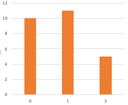
The examples I gave in that article were continuous distributions, but this technique works equally well with discrete distributions. (For discrete quantities we call the “probability distribution” function the “probability mass” function, for no particularly good reason I’m aware of.)  In our case today we can simply treat the mass function as a non-normalized distribution. Here’s the non-normalized mass function for weights 10, 11, 5.

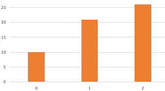
• Since the mass function is just a bunch of integer weights for integer values, the cumulative distribution function is a monotone step function, also from integers to integers. Here’s the cumulative distribution, which is 10, 21, 26.  (That is, 10, 10+11, 10+11+5.)

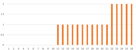
• The quantile function is the inverse of that function, which is another step function from integers to integers. Here’s the quantile function:

• We just evaluate that function at a uniformly random point, and we’re done.  That is, we pick a uniform integer from 1 to 26, and look at the quantile function. If it is 1 through 10, we choose zero. If it is 11 through 21, we choose one, and if it is 22 through 26, we choose 2.

We get a number out from 0, 1 and 2 at the ratios of 10:11:5, as desired. And we did everything in integers; no pesky double arithmetic to get in the way. Are we done?

Sadly, no; the question is thoroughly begged! We already knew how to do that; we just create an array with ten zeros, eleven ones and five twos and sample from it. We’re trying to avoid that solution.

But maybe we can use these ideas to come up with a more efficient way to do the same thing.

The first thing we’ll do is compute the cumulative distribution in the constructor:

private readonly List<int> cumulative;
private WeightedInteger(List<int> weights)
{
  this.weights = weights;
  this.cumulative = new List<int>(weights.Count);
  cumulative.Add(weights[0]);
  for (int i = 1; i < weights.Count; i += 1)
    cumulative.Add(cumulative[i – 1] + weights[i]);
}

So, if we start with weights 10, 11, 5, we have cumulative weights 10, 21, 26.

Again, remember what this means. Based on the weights, the probability of getting 0 is 10/26, the probability of getting 1 is 11/26, and the probability of getting 2 is 5/26.  Therefore the probability of getting 0 or less is 10/26, the probability of getting 1 or less is 21/26, and the probability of getting 2 or less is 26/26. That’s how we compute the weights of the cumulative distribution.

Now we need to invert that cumulative distribution function. That is the function q(x) where q(1 to 10) = 0, q(11 to 21) = 1, q(22 to 26) = 2. We need to generate a random integer, and then compute this function, but how do we compute this function?

We generate a random number from 1 to 26, and then search the cumulative list for it. We’ll do a linear search for the leftmost bucket where the cumulative weight is not less than the sample:

public int Sample() 
{
  int total = cumulative[cumulative.Count – 1];
  int uniform = SDU.Distribution(1, total).Sample();
  int result = 0;
  while (cumulative[result] < uniform)
    result += 1;
  return result;
}

You can verify for yourself that if we sample 1-10 we get 0, if we sample 11-21 we get 1, and if we sample 22-26 we get 2.

Is that it? Can it really be that easy? I think it can, but let’s try it out:

WeightedInteger.Distribution(10, 11, 5).Histogram()

0|************************************
1|****************************************
2|******************

Looking good!

Obviously it is O(n) to compute the cumulative weights, but we only have to do that once, in the constructor. The more worrisome problem is that searching for the result is O(n) in the number of weights.

If the number of weights is three or five or twenty, it’s probably not a problem. But if it’s a hundred or a thousand, a linear search is going to be problematic. (Then again, if it is more than a thousand, our assumption that discrete distributions have a small support is probably going out the window too.)

But of course we know how to improve the search time when we’re looking for an item in a sorted list; we can binary search it! As the documentation notes, the BinarySearch method of List returns “the zero-based index of item in the sorted list, if item is found; otherwise, a negative number that is the bitwise complement of the index of the next element that is larger than item…” which is exactly what we want.

• If we generate 10, 21 or 26 then we get the result we want immediately: 0, 1 or 2.
• If we generate 1 through 9, we get ~0, because cumulative[0] is larger
• similarly 11 through 20 gives us ~1
• similarly 22 through 25 gives us ~2

But ~ is its own inverse, so we can just ~ the result if negative and get the answer we want. Let’s implement it:

public int Sample() 
{
  int total = cumulative[cumulative.Count – 1];
  int uniform = SDU.Distribution(1, total).Sample();
  int result = cumulative.BinarySearch(uniform);
return result >= 0 ? result : ~result;
}

Seems legit.

Right?

Hmm.

Exercise: There’s a bug in the code above. Do you see it?

Give it some thought and then scroll down.

.

.

.

.

.

.

.

.

.

Since we are no longer looking “from the left”, we can accidentally choose a bucket that has a zero probability. For example, if our weights are 10, 0, 0, 11, 5, then the cumulative weights are 10, 10, 10, 21, 26. If 10 is our uniform sample then we must ensure that the binary search finds the leftmost 10 and says “0”, and not “1” or “2”.

There are a variety of techniques you could employ to solve this problem efficiently, and I’m not going to dig into them here. Give it a shot!

Let’s assume that we managed to solve our binary searching bug. This reduces our cost from O(n) to O(log n) which is very good, and for practical purposes, probably good enough. After all, with a thousand weights, that’s at most 10 comparisons, which should be pretty quick.

However, let’s think about some pathological cases.

Suppose we have a probability distribution with a thousand elements, distributed like this: 1, 1, 1, 1, 1, …. 1, 1001. The cumulative distribution will be 1, 2, 3, … 999, 2000. But  50% of the time on average we will uniformly generate a number greater than 999 and less than 2000, so 50% of the time our binary search will have to do all ten comparisons to discover that the rightmost bucket is the one we want. Can we do better?

Yes we can. Instead of building a list and binary searching that, we could build an optimal binary search tree and search that. We know ahead of time the probability of choosing each element in the binary search tree, so we can move the most common buckets towards the root of the tree, and then build a balanced binary search tree for the uncommon items in the leaves; there is an O(n²) algorithm for doing so, but I’m not going to show it here; see the Wikipedia article for details.

Alternatively, we could use a self-tuning binary tree such as a splay tree, and have it reorganize itself so that the most commonly searched for buckets appear near the root.

If we pursued this option of building a binary search tree, we could also prune zero-probability buckets from the tree entirely, eliminating the problem I mentioned above of accidentally finding a zero-probability bucket.

By using these techniques, we can get the average time spent sampling very low indeed, even for pathological cases, but it will still take longer to sample as the number of weights increases. (And we have a potentially difficult quadratic algorithm to build the optimized tree, though that only happens once.) Can we find a simple algorithm where the sample time is constant no matter how many weights there are?

Next time on FAIC: We’ll make two more attempts to find a more efficient sampling technique for this distribution.

[Code is here.]

Last time on FAIC I showed how we could implement more of the standard, straightforward probability distributions, like the Bernoulli distribution; the episode before I showed the standard discrete uniform distribution, also known as “roll an n-sided fair die”. But typically when we are working on a line-of-business program, we’re working on objects that are meaningful in that line of business, and not necessarily on integers. Just to pick a silly example, suppose I want to uniformly choose between a cat, a dog and a goldfish?

using SDU = StandardDiscreteUniform;
…
var animals = new List<Animal>()
  { new Cat(), new Dog(), new Goldfish() };

Traditionally, as I noted a while back, we’d write some mechanism-heavy code like:

var choice = animals[random.Next(0, animals.Length)];

Now, I sincerely hope you’re not satisfied with:

var choice = animals[
  SDU.Distribution(0, animals.Length-1).Sample()];

If I tried to push that nonsense on you, you’d be quite justified in concluding that this whole project of mine to motivate a better “Random” is a cure that is worse than the disease. As is often the case, the problem here is that we’ve failed to push the “mechanism” code into a helper class, so let’s do that:

// This is wrong!
public sealed class DiscreteUniform<T> :
  IDiscreteDistribution<T>
{
  private readonly SDU sdu;
  private readonly List<T> support;
  public static DiscreteUniform<T> Distribution(
      IEnumerable<T> items) =>
    new DiscreteUniform<T>(items);
  private DiscreteUniform(IEnumerable<T> items)
  {
    this.support = items.ToList();
    this.sdu = SDU.Distribution(0, support.Count – 1);
  }
  public IEnumerable<T> Support() => support;
  public T Sample() => support[sdu.Sample()];
  public int Weight(T t) => this.support.Contains(t) ? 1 : 0;
  public override string ToString() =>
    $”DiscreteUniform[{string.Join(“,”, support)}]”;
}

Exercise: That code is wrong in a number of ways; what are they? Give it some thought and then scroll down.

.

.

.

.

.

.

1. We do not handle the case where the sequence is empty, which should be an error, or a single item, which would be better represented as a Singleton<T>.
2. A buggy or hostile caller could call Support(), cast it to List<T>, and then mutate the list. Defense in depth!
3. Suppose the array contains two references to the same dog, and a cat and a fish. If we ask what the weight is for the cat, we get 1; if we ask what the weight of the dog is, we get 1, but the dog is twice as likely to be chosen.
4. Also in that scenario: the support contains the same dog twice. We expect the support to contain exactly one of each possible value.

We’ll fix all these problems in our final implementation at the bottom of this post.

Suppose we’ve managed to fix the problems identified above. We now create a helper method:

public static IDiscreteDistribution<T> ToUniform<T>(
    this IEnumerable<T> items) =>
  DiscreteUniform<T>.Distribution(items);

And now our proposed code is much nicer:

var animals = new List<Animal>()
  { new Cat(), new Dog(), new Goldfish() };
var choice = animals.ToUniform().Sample();

That looks much nicer, but… I still don’t like it.

Oh, sure, I like the call site, with the beautiful, readable fluent extension methods and whatnot. What I don’t like is the fact that I just built yet another single-purpose wrapper class. This wrapper class is only good for making a uniform distribution of an arbitrary sequence. Suppose I have a non-uniform distribution of integers from 0 to n — say, a binomial distribution — and I want to map a list of animals to that distribution; am I going to have to write a “binomial distribution on sequence” class that duplicates almost all the logic of the wrapper class above?

Exercise: Implement the binomial distribution; this is the extension of the Bernoulli distribution where, again, we have weights for a possibly-unfair coin, but we also have a parameter n which is the number of coin flips to make. The result is the total number of heads. Sampling is straightforward, but can you see how to compute the weights?

This seems like an opportunity for a more sophisticated wrapper class, parameterized in the underlying distribution on integers. Let’s tweak the class we just wrote:

public sealed class IntegerDistributionWrapper<T> :
  IDiscreteDistribution<T>
{
  private readonly IDiscreteDistribution<int> d;
  private readonly List<T> items;
  public static IntegerDistributionWrapper<T> Distribution(
    IDiscreteDistribution<int> d,
    IEnumerable<T> items)
{
    // blah blah blah
  }
  private IntegerDistributionWrapper(
    IDiscreteDistribution<int> d,
    IEnumerable<T> items)
  {
// you get the idea
  }
  public T Sample() => items[d.Sample()];
// and so on

I waved my hands a lot there because, though this is an improvement, I still don’t like it. We’re getting better, but I want more generality for less cost. What are we doing here really?

• Sampling an integer from a distribution.
• Projecting that integer onto a value taken from a list.

Why does the projection have to be “value taken from a list”? And for that matter, why does the value sampled from the underlying distribution have to be an integer to begin with? We can write almost the same code, but make it far more general:

public sealed class Projected<A, R> :
  IDiscreteDistribution<R>
{
  private readonly IDiscreteDistribution<A> underlying;
  private readonly Func<A, R> projection;
  private readonly Dictionary<R, int> weights;
  public static IDiscreteDistribution<R> Distribution(
    IDiscreteDistribution<A> underlying,
    Func<A, R> projection)
  {
    var result = new Projected<A, R>(underlying, projection);
    if (result.Support().Count() == 1)
      return Singleton<R>.Distribution(
        result.Support().First());
    return result;
  }
  private Projected(
    IDiscreteDistribution<A> underlying,
    Func<A, R> projection)
  {
    this.underlying = underlying;
    this.projection = projection;
    this.weights = underlying.Support().
      GroupBy(
        projection, 
        a => underlying.Weight(a)).
      ToDictionary(g => g.Key, g => g.Sum());
  }
  public R Sample() => projection(underlying.Sample());
  public IEnumerable<R> Support() => this.weights.Keys;
  public int Weight(R r) =>
    this.weights.GetValueOrDefault(r, 0);
}

Study that implementation and make sure it makes sense to you; the crux of the whole thing is in the constructor, where we compute the weights of the resulting distribution.

You’ve probably noticed that I’ve fixed all the problems identified above:

• We return a singleton when possible
• We don’t need to worry about the distribution being empty because presumably the underlying distribution is not empty
• The support set is an immutable deduplicated keyset
• We compute the weights up front.

Unfortunately this means O(support) extra storage, but I can live with that.

Exercise: there are a number of optimizations that could be made here for the common case where the number of “colliding” elements in the support is small or zero, to reduce the amount of extra storage. Try implementing some of them, see if you get a win.

Now that we have a projection wrapper, we can delete our discrete uniform wrapper and integer wrapper classes entirely. That means we have to rewrite our helper method:

public static IDiscreteDistribution<T> ToUniform<T>(
  this IEnumerable<T> items)
{
  var list = items.ToList();
  return Projected<int, T>.Distribution(
    SDU.Distribution(0, list.Count – 1),
    i => list[i]);
}

But again, this seems like I’m missing some generality.

Hmm.

Maybe I should also write an extension method on distributions that makes a projected distribution. It’s an easy helper method after all:

public static IDiscreteDistribution<R> MakeProjection<A, R>(
    this IDiscreteDistribution<A> d,
    Func<A, R> projection) =>
  Projected<A, R>.Distribution(d, projection);

Wait a minute… that looks very familiar.

Scroll down when you see it.

.

.

.

.

.

.

.

Good heavens, we’ve re-invented Select. Again. 

public static IDiscreteDistribution<R> Select<A, R>(
    this IDiscreteDistribution<A> d,
    Func<A, R> projection) =>
  Projected<A, R>.Distribution(d, projection);

And now this helper can be rewritten into a call to Select:

public static IDiscreteDistribution<T> ToUniform<T>(
  this IEnumerable<T> items)
{
  var list = items.ToList();
  return SDU.Distribution(0, list.Count – 1)
    .Select(i => list[i]);
}

But you know what this means: I have a Select method with the right signature, which means I can use my beloved query comprehension syntax! That last line could be

return
  from i in SDU.Distribution(0, list.Count – 1)
  select list[i];

And now you know why, a few episodes back I said that I was not going to make IDistribution<T> an extension of IEnumerable<T>; doing so just causes confusion between the Select operation on distributions and the Select operation on sequences.

Aside: If you’ve been following along you’ve noticed that this implementation takes a list, then turns it into a list, and then turns it into a list again, and then turns it into a dictionary. This seems “not cheap”. And indeed it is not, but remember, this is pedagogical code, not industrial code. Were I writing this library for industry, I’d be optimizing it much more to avoid collection pressure.

The idea here is to sketch out what could be done, not exactly how we’d do it. When I think about performance in this series, I’m going to be concentrating on things like eliminating arbitrarily expensive loops, and not on pragmatic but mundane practicalities like eliminating sources of collection pressure.

Finally, let’s just make sure that everything is working as expected:

var cat = new Cat();
var dog = new Dog();
var fish = new Goldfish();
var animals = new List<Animal>() { cat, dog, dog, fish };
Console.WriteLine(animals.ToUniform().Histogram());
Console.WriteLine(animals.ToUniform().ShowWeights());

Sure enough, we get the correct distribution:

     Cat|*******************
     Dog|****************************************
Goldfish|*******************
     Cat:1
     Dog:2
Goldfish:1

Interesting! We started by trying to make a uniform distribution and ended up with a correct non-uniformly-weighted distribution. Can we do a better job of building such a distribution without having to make an array that has duplicates?

Next time on FAIC: we’ve already seen how to represent a “fair die roll” distribution and a Bernoulli distribution where we give the “odds” that either zero or one happens as a ratio of integers; we’ll extend those concepts to any number of weighted outcomes, and discuss what data structure we can use to efficiently sample that distribution.

[Code is here.]

Last time on FAIC I implemented our first discrete distribution, the “choose an integer between min and max” distribution. I thought I might knock out a couple more of the easy discrete distributions. The easiest discrete distribution of all is of course the trivial distribution:

public sealed class Singleton<T> : IDiscreteDistribution<T>
{
  private readonly T t;
  public static Singleton<T> Distribution(T t) =>
    new Singleton<T>(t);
  private Singleton(T t) => this.t = t;
  public T Sample() => t;
  public IEnumerable<T> Support()
  {
    yield return t;
  }
  public int Weight(T t) =>
EqualityComparer<T>.Default
.Equals(this.t, t) ? 1 : 0;
  public override string ToString() =>
    $”Singleton[{t}]”;
}

That is, the probability distribution where 100% of the time it returns the same value. You’ll also sometimes see distributions like this called the “Dirac delta” or the “Kronecker delta”, but we’re not doing quantum physics here, so I’m going to just call this the singleton distribution and be done with it.

Aside: I wish the Enumerable class had the corresponding method: take an item, return the sequence containing only that item. As we just saw, it’s easy to implement; because it is not in the framework, I’ve implemented it literally dozens of times! It is weird to me that the “extract the value of a singleton sequence” is a member of Enumerable, but the inverse operation is not.

Aside: This is the first distribution we’ve seen that does not necessarily have some sort of number as its output. You might be thinking that maybe our distribution type should never have been generic in the first place, if the only distributions I’m going to come up with are either numeric-valued or trivial. But worry not! In the next episodes we’ll see how we can naturally use more complex types in probability distributions.

Let’s look at another integer-valued distribution. The Bernoulli distribution considers the question “what if we flipped a possibly-unfair coin, and scored 1 for a head and 0 for a tail?” The parameter to the distribution is traditionally the probability of heads in our  coin, between 0.0 and 1.0. However, as I noted last time, at least for now I’m going to try to avoid double weights. Instead, we’ll think of this distribution as “odds”. Instead of saying “0.7 chance of getting a 1”, we’ll say “we get three zeros for every seven ones”:

public sealed class Bernoulli :
  IDiscreteDistribution<int>
{
  public static IDiscreteDistribution<int> Distribution(
    int zero, int one)
  {
    if (zero < 0 || one < 0 || zero == 0 && one == 0)
      throw new ArgumentException();
    if (zero == 0) return Singleton<int>.Distribution(1);
    if (one == 0) return Singleton<int>.Distribution(0);
    return new Bernoulli(zero, one);
  }
  public int Zero { get; }
  public int One { get; }
  private Bernoulli(int zero, int one)
  {
    this.Zero = zero;
    this.One = one;
  }
  public int Sample() =>
    (SCU.Distribution.Sample() <=
      ((double)Zero) / (Zero + One)) ? 0 : 1;
  public IEnumerable<int> Support() =>
    Enumerable.Range(0, 2);
  public int Weight(int x) => x == 0 ? Zero : x == 1 ? One : 0;
  public override string ToString() =>
    $”Bernoulli[{this.Zero}, {this.One}]”;
}

And sure enough, if we graph it out:

Bernoulli.Distribution(1, 3).Histogram()

We get what you’d expect: three times as many heads as tails:

0|*************
1|****************************************

Next time on FAIC: We’ll stop making new implementations of classic probability distributions and look at how to extend the ones we’ve got.

[Code is here.]

Last time on FAIC I showed how we could use a simple interface to cleanly implement concepts like “normal distribution” or “standard uniform distribution” in a natural style using fluent programming. For the next many episodes we’ll leave continuous distributions aside and consider only discrete distributions. That is, we have some probability distribution where there are only a small, fixed number of outcomes. Flip a coin, roll three dice and add them together, that sort of thing.

Since we assume the number of possible outcomes of a discrete distribution is small, we can enumerate them; the set of possible outcomes is, oddly enough, called the support of the distribution.

Some elements might be more likely than others; the ones that happen more often we say have more weight than the ones that happen less often. I want to be able to describe the weight of each member of a distribution easily, and I do not want to get off in the weeds of representing weights as doubles because double arithmetic has many pitfalls as we well know. For the purposes of this series I’m going to assume that we can weight the members of a distribution by an integer. (If I get around to it I might discuss double-weighted distributions later on.)

public interface IDiscreteDistribution<T> : IDistribution<T>
{
  IEnumerable<T> Support();
  int Weight(T t);
}

I’m going to require that the weight function accept any value of type T. If the value is not in the support, the weight is zero, and if the value is in the support, the weight is a positive integer. I’m going to further assume that the support and weights are small enough that the total weight fits into an integer.

Aside: If you divide the weight function by the total weight (as a double) then you have the probability mass function of the discrete distribution.

I said way back in part one of this series that System.Random has a “candy-machine interface” problem. Let’s solve that problem right now:

using SCU = StandardContinuousUniform;
public sealed class StandardDiscreteUniform :
  IDiscreteDistribution<int>
{
  public static StandardDiscreteUniform Distribution(
    int min, int max)
  {
    if (min > max)
      throw new ArgumentException();
    return new StandardDiscreteUniform(min, max);
  }
  public int Min { get; }
  public int Max { get; }
  private StandardDiscreteUniform(int min, int max)
  {
    this.Min = min;
    this.Max = max;
  }
  public IEnumerable<int> Support() =>
    Enumerable.Range(Min, 1 + Max – Min);
  public int Sample() =>
    (int)((SCU.Distribution.Sample() *
      (1.0 + Max – Min)) + Min);
  public int Weight(int i) =>
(Min <= i && i <= Max) ? 1 : 0;
  public override string ToString() =>
    $”StandardDiscreteUniform[{Min}, {Max}]”;
}

Finally we can now do things like 10d6 (D&D notation for “sum ten six-sided die rolls”) in a natural, fluent style. I would far prefer:

SDU.Distribution(1, 6).Samples().Take(10).Sum()

to

random.Next(1, 7) + random.Next(1, 7) + random.Next(1, 7) + …

or the equivalent loop nonsense that you typically see.

A common defense of “lower bound inclusive, upper bound exclusive” is that it is natural for programmers in C-family languages to think of an array or list as indexed from 0 (inclusive) to the array length (exclusive). Apparently we want to be able to say things like

myArray[Random.Next(0, myArray.Length)]

and not get confused and have to say myArray.Length-1.  Well, my answer to that (germane) critique is: once again, we’re reasoning at the wrong level. If we want a probability distribution drawn from elements of an array, then don’t mess around with array indexing and choosing the right random number and so on. That is writing code at the level of the mechanisms, not the business domain. Instead, make an object that represents a distribution of elements chosen from a given array and sample from it!

But we are getting ahead of ourselves; we’ll get to that in an upcoming episode.

Previously I made a little “histogram string” helper extension method that is useful for quickly displaying results in a debugger or console; let’s do the same for discrete distributions. Moreover, to make sure that we really are getting the results we expect, I’m going to implement it by sampling rather than just basing it on the support and the corresponding weights:

public static string Histogram<T>(
  this IDiscreteDistribution<T> d) =>
  d.Samples().DiscreteHistogram();

public static string DiscreteHistogram<T>(
  this IEnumerable<T> d)
{
  const int sampleCount = 100000;
  const int width = 40;
  var dict = d.Take(sampleCount)
    .GroupBy(x => x)
    .ToDictionary(g => g.Key, g => g.Count());
  int labelMax = dict.Keys
    .Select(x => x.ToString().Length)
    .Max();
  var sup = dict.Keys.OrderBy(x => x).ToList();
  int max = dict.Values.Max();
  double scale = max < width ? 1.0 : ((double)width) / max;
  return string.Join(“\n”,
    sup.Select(s => $”{ToLabel(s)}|{Bar(s)}“));
  string ToLabel(T t) =>
    t.ToString().PadLeft(labelMax);
  string Bar(T t) =>
    new string(‘*’, (int)(dict[t] * scale));
}

I gotta say, I am loving local functions in C# 7.

Let’s take it for a test drive and roll 1d10:

StandardDiscreteUniform.Distribution(1, 10).Histogram()

The histogram appears as we’d expect:

 1|***************************************
 2|***************************************
 3|***************************************
 4|**************************************
 5|***************************************
 6|****************************************
 7|**************************************
 8|***************************************
 9|***************************************
10|**************************************

Of course, sometimes we will want to see the weights directly:

public static string ShowWeights<T>(
  this IDiscreteDistribution<T> d)
{
  int labelMax = d.Support()
    .Select(x => x.ToString().Length)
    .Max();
  return string.Join(“\n”, d.Support().Select(s =>
    $”{ToLabel(s)}:{d.Weight(s)}“));
  string ToLabel(T t) =>
    t.ToString().PadLeft(labelMax);
}

We seem to be doing pretty well here; our implementations of each probability distribution are short and sweet, and each one provides a stone in the foundation for building more complex distributions.

Next time on FAIC: we’ll build more simple discrete distributions.