Happy New Year all!
Last time I briefly described the basic strategy of the Beanstalk compiler: transform the source code of each queried or observed function (and transitively their callees) into an equivalent program which partially evaluates the model, accumulating a graph as it goes. In this post I’ll go through the first step of the transformation.
The idea of the first source-to-source transformation is to take a relatively complicated language — Python — and replace it with what I think of as “simplified Python”. The Zen of Python famously says “there should be one — and preferably only one — obvious way to do it” but that is not the goal of this simplification step. The Zen of Python emphasizes obviousness. It is about making the code clear and the language discoverable. My goal with simplified Python is “there should be only one way to do it” — because it is easier to instrument a program to capture its meaning as it runs if there’s only one way to do everything.
Consider for example how to call a function foo with three arguments:
foo(1, 2, 3)
x = [1, 2, 3]
foo(*x)
foo(1, 2, bar=3)
x = {"bar":3}
foo(1, 2, **x)
… and so on — there are a great many obvious ways to call a function in Python, but I’d like there to be exactly one in simplified Python.
The first thing we do when analyzing a queried or observed function is to obtain its source code, parse that into an abstract syntax tree (AST), and then do a series of AST transformations that reduce the function into an equivalent but simpler Python program. This is the most traditional-compiler-ish step in the pipeline.
(How do we obtain the source code? Remember, we have an RVID for each observation and query; the RVID contains a reference to the original function object. Python’s runtime can provide the source code for a given function reference.)
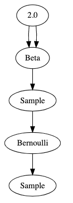
Let’s look at an only slightly more complicated version of our “hello world” model:
@random_variable
def fairness():
  return Beta(2,2)

@random_variable
def flip(n):
  return Bernoulli(0.5 * fairness())
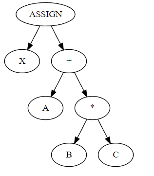
In our simplified Python:
- Every value gets its own variable
- Every computation gets its own statement
- Every call has the same syntax:
a = b(*c, **d)
Our two methods in the simplified form would be:
def fairness():
  _t1 = 2
  _t2 = 2
  _t3 = [_t1, _t2]
  _t4 = {}
  _t5 = Beta(*_t3, **_t4)
  return _t5

def flip(n):
  _t1 = 0.5
  _t2 = []
  _t3 = {}
  _t4 = fairness(*_t2, **_t3)
  _t5 = _t1 * t4
  _t6 = [_t5]
  _t7 = {}
  _t8 = Bernoulli(*_t6, **_t7)
  return _t8
ASIDE: Readers with some experience writing compilers might ask “is this static-single-assignment form?” SSA form is a transformation whereby every variable is assigned exactly once; it’s used for control flow analysis and other program analyses. I did not write a full-on SSA transformation but when I was doing initial prototyping I knew that I might need SSA form in the future. Think of it as SSA-light if that makes sense.
We can go further; in our simplified Python:
- logical operators
andandorare eliminated
x = y and z
can be simplified to
x = y
if x:
  x = z
and now the graph accumulator does not need to worry at all about logical operators, because there aren’t any in the simplified program.
- Every
whileloop iswhile True.
- No loop has an
elseclause. (Did you know that Python loops haveelseclauses? It’s true!)
- There are no compound comparisons:
x = a < b < c
can be simplified to
x = a < b
if x:
  x = b < c
and now the graph accumulator does not need to worry about compound comparisons, because there aren’t any.
- Similarly there are no lambdas, no function annotations, and so on. All the convenient syntactic sugars are desugared into their more fundamental form.
The simplified language is definitely not a language I’d like to write a long program in, but it is a language that is easy to analyze programmatically. Thus far, the transformations make the program longer and simpler, but do not change its meaning; if we compiled and ran the simplified version of the program it should do the same thing as the normal version.
Next time on FAIC: let’s get into the details of how the AST-to-AST transformation code works. I had a lot of fun writing it.