Today, yet another episode in my ongoing series “What’s the difference?” This time, a non-computer-related topic.
I am often complimented on my choice of outerwear in the Seattle rainy season, and I hate to respond to a well-meant compliment with a correction. So I usually let all those “Nice trenchcoat!” comments slide and just say “Thanks!” But as a public service, let me lay it out for you so that you don’t make the same mistake. Here we see David Tennant as the Tenth Doctor wearing a classic example of a trenchcoat: (Click for a larger version.)
The trenchcoat is a long waterproof coat, traditionally made of gabardine. The term originated in the trenches of the First World War, due to the popularity of this style of coat amongst officers in the British armed forces. The trench coat is not merely a functional warm raincoat but also stylish, with long wide lapels and decorative buttons. The trenchcoat is often belted and might be tailored in at the waist, particularly for women’s trenchcoats.
A duster is also a long waterproof coat that is often referred to as a “trenchcoat” — but as you’ll see, it is quite different in its details. Here’s the duster I wear, an Australian-made Driza-Bone:
Note the lack of decorative elements, the flap over the closure, the no-lapel collar (which clasps shut, completely enclosing the neck if necessary) and the built-in extra rain protection on the shoulders. (*) Dusters are typically made of oilcloth and are built for handling the practicalities of herding sheep in the rain, not for style (**).
Not shown in this view: the interior includes straps that let you attach the bottom of the coat to your legs, so that it does not blow around when you are on horseback. Also, the back is cut in such a way that you can cover both your legs and the rear portion of the saddle with the coat. I usually take the bus and not a horse to work, but still it’s nice to know that options are available should I need them. These practical elements are usually not present in trenchcoats.
(*) Duster manufacturers always hasten to point out that the shoulders are already waterproof; the extra layer keeps your shoulders warmer by shedding rain more effectively.
(**) There are, of course, some dusters built for style; if you watch the “Matrix” series of movies you’ll see the heroes wear an assortment of extremely stylish dusters and trenchcoats both.
If you ask a dozen C# developers what a “local variable” is, you might get a dozen different answers. A common answer is of course that a local is “a storage location on the stack”. But that is describing a local in terms of its implementation details; there is nothing in the C# language that requires that locals be stored on a data structure called “the stack”, or that there be one stack per thread. (And of course, locals are often stored in registers, and registers are not the stack.)
A less implementation-detail-laden answer might be that a local variable is a variable whose storage location is “allocated from the temporary store”. That is, a local variable is a variable whose lifetime is known to be short; the local’s lifetime ends when control leaves the code associated with the local’s declaration space.
That too, however, is a lie. The C# specification is surprisingly vague about the lifetime of an “ordinary” local variable, noting that its lifetime is only kinda-sorta that length. The jitter’s optimizer is permitted broad latitude in its determination of local lifetime; a local can be cleaned up early or late. The specification also notes that the lifetimes of some local variables are necessarily extended beyond the point where control leaves the method body containing the local declaration. Locals declared in an iterator block, for instance, live on even after control has left the iterator block; they might die only when the iterator is itself collected. Locals that are closed-over outer variables of a lambda are the same way; they live at least as long as the delegate that closes over them. And in the upcoming version of C#, locals declared in async blocks will also have extended lifetimes; when the async method returns to its caller upon encountering an “await”, the locals live on and are still there when the method resumes. (And since it might not resume on the same thread, in some bizarre situations, the locals had better not be stored on the stack!)
So if locals are not “variables on the stack” and locals are not “short lifetime variables” then what are locals?
The answer is of course staring you in the face. The defining characteristic of a local is that it can only be accessed by name in the block which declares it; it is local to a block. What makes a local truly unique is that it can only be a private implementation detail of a method body. The name of that local is never of any use to code lexically outside of the method body.
Here’s an inconvenient truth: just about every “public surface area” change you make to your code is a potential breaking change.
First off, I should clarify what I mean by a “breaking change” for the purposes of this article. If you provide a component to a third party, then a “breaking change” is a change such that the third party’s code compiled correctly with the previous version, but the change causes a recompilation to fail. (A more strict definition would be that a breaking change is one where the code recompiles successfully but has a different meaning; for today we will just consider actual “build breaks”.)
A “potential” breaking change is a change which might cause a break, if the third party happens to have consumed your component in a particular way. By a “public surface area” change, I mean a change to the “public metadata” surface of a component, like adding a new method, rather than changing the behaviour of an existing method by editing its body. (Such a change would typically cause a difference in runtime behaviour, rather than a build break.)
Some public surface area breaking changes are obvious: making a public method into a private method, sealing an unsealed class, and so on. Third-party code that called the method, or extended the class, will break. But a lot of changes seem a lot safer; adding a new public method, for example, or making a read-only property into a read-write property. As it turns out, almost any change you make to the public surface area of a component is a potential breaking change. Let’s look at some examples. Suppose you add a new overload:
// old component code:
public interface IFoo {...}
public interface IBar { ... }
public class Component
{
    public void M(IFoo x) {...}
}
The consumer code compiles successfully against the original component, but recompiling it with the new component suddenly the build breaks with an overload resolution ambiguity error. Oops.
What about adding an entirely new method?
// old component code:
...
public class Component
{
  public void MFoo(IFoo x) {...}
}
and now you add
public void MBar(IBar x) {...}
No problem now, right? The consumer could not possibly have been consuming MBar. Surely adding it could not be a build break on the consumer, right?
class Consumer
{
    class Blah
    {
        public void MBar(IBar x) {}
    }
    static void N(Action<Blah> a) {}
    static void N(Action<Component> a) {}
    static void D(IBar bar)
    {
        N(x=>{ x.MBar(bar); });
    }
}
Oh, the pain.
In the original version, overload resolution has two overloads of N to choose from. The lambda is not convertible to Action<Component> because typing formal parameter x as Component causes the body of the lambda to have an error. That overload is therefore discarded. The remaining overload is the sole applicable candidate; its body binds without error with x typed as Blah.
In the new version of Component the body of the lambda does not have an error; therefore overload resolution has two candidates to choose from and neither is better than the other; this produces an ambiguity error.
This particular “flavour” of breaking change is an odd one in that it makes almost every possible change to the surface area of a type into a potential breaking change, while at the same time being such an obviously contrived and unlikely scenario that no “real world” developers are likely to run into it. When we are evaluating the impact of potential breaking changes on our customers, we now explicitly discount this flavour of breaking change as so unlikely as to be unimportant. Still, I think its important to make that decision with eyes open, rather than being unaware of the problem.
This article elicited many reader comments:
You pretty much have to ignore these possible problems, the same way you can’t guess what extension methods we’ve made that may be silently overridden by new methods in a class.
That was our conclusion, yes.
Could you give an example where making a read-only property into a read-write property would result in a breaking change? I can’t think of any…
Sure:
class C { public int P { get; set; } }
class D { public int P { get; private set; } }
class E {
  static void M(Action<C> ac){}
  static void M(Action<D> ad) {}
  static void X() { M(q=>{q.P = 123; }); }
}
The body of X binds without error as long as D.P‘s setter is private. If it becomes public then the call to M is ambiguous.
I’m curious to see how unsealing a class can cause code to stop compiling.
Same trick. This trick is surprisingly versatile.
class B {}
sealed class C {}
class D : B, I {}
interface I {}
class P {
  static void M(Func<C, I> fci){}
  static void M(Func<B, I> fbi){} // special agent!
  static void Main() { M(q=>q as I); }
}
That compiles successfully because q as I is illegal if q is of type C. The compiler knows that C does not implement I, and because it is sealed, it knows that no possible type that is compatible with C could implement I. Therefore overload resolution chooses the func from B to I, because a derived type B, say, D, could implement I. When C is unsealed then overload resolution has no basis to choose one over the other, so it becomes an ambiguity error.
Seems to me you would be much better off in this regard avoiding the new functional features and sticking to the C# 2.0 specifications. That way you’re pretty much protected against breakages like these right?
At what cost? Is it worthwhile to eschew the benefits of LINQ in order to avoid the drawbacks of some obscure, unlikely and contrived breaking changes? The benefits of LINQ outweigh the costs by a huge margin, in my opinion.
You know, all these examples make me think overload resolution is just too clever for its own good — these kinds of algorithms are more the kind you’d expect in the optimizing part, where cleverness abounds, not in the basic semantic part. Clearly, the solution is to abolish overload resolution, assign every method an unambiguous canonical name (that’s stable in the face of changes) and force the developer to specify this name on every call. Alternatively, make overload resolution unnecessary by forbidding overloads. Not sure how to handle generics in such a world — abolishing them seems too harsh. (Mandatory Internet disclaimer: the above is facetious, but slightly ha-ha-only-serious.)
There are languages that do not have overload resolution. A .NET language could, for instance, specify the unique metadata token associated with the method definition. But in a world without overload resolution, how would you do query comprehensions?
Before we get started, thanks for all the great comments to the previous couple of posts. I’ll be updating the algorithm to try to make even better-looking circles of light based on the comments. Like I said, there’s a lot of subtleties to these algorithms and I am just learning about them myself.
To that end, in today’s episode I am going to spend the entire prolix article analyzing a single division operation. You have been warned.
Before we begin though, some jargon. A cell which is invisible that by our physical interpretation ought to be visible, or a cell which is visible that ought to be invisible we will call an “artifact”. An “artifact” is the product of our algorithm (or some detail of its implementation) not being a sufficiently accurate model of real-world physics. Today’s article will be all about artifacts.
The actual workhorse that implements the field-of-view algorithm is this method that we mentioned last time:
private static void ComputeFoVForColumnPortion(
int x,
DirectionVector topVector,
DirectionVector bottomVector,
Func<int, int, bool> isOpaque,
Action<int, int> setFieldOfView,
int radius,
Queue<ColumnPortion> queue)
{
This method has two main purposes. First, it assumes that all points in the portion of column x bounded by the top and bottom vectors are in the field of view, and marks them accordingly; some of them might be outside the radius, but the rest of them are by assumption visible from the origin. Second, it determines which portions of column x+1 are in the field of view and adds them to the work queue for later processing.
We described the algorithm as working from top to bottom of the portion of the column under consideration. Therefore the very first question we must answer is “which exactly is the top cell in the column portion, given the column number and the top direction vector?”
If the center point of a cell in column x happens to fall exactly on the top direction vector then it is pretty clear which is the top cell. Suppose for the sake of argument that’s the case. The top cell is then computed by x * topVector.Y / topVector.X. This division is exact. Proving that is an easy bit of algebra and is left as an exercise.
So perhaps we should say that even if the division is inexact, we compute the top cell by:
int topY = x * topVector.Y / topVector.X;
(Note that we’ll assume throughout that the numbers we are multiplying and dividing are small compared to the range of int, and therefore do not overflow.)
What happens if the division is inexact? We know that in C# an inexact integer division always rounds towards zero; it rounds down if necessary.
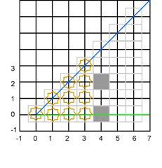
Rounding down is a bad idea because it doesn’t model the physical world well and makes for extraordinarily bad-looking gameplay. Consider this extremely common scenario:
Scenario One
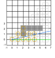
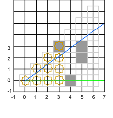
After processing column one we lower the slope of the top direction vector to one-third. Is point (2,1) in the field of view? It sure seems light it ought to be since its entire bottom surface is within the field of view. But if we do 2 * 1 / 3 we get zero, so no, the top cell that is visible in this column is (2, 0). We mark that as visible and continue on to column three without changing the slope. The top direction vector now intersects the center of cell (3, 1), so it and (3, 0) are visible. We lower the slope of the top vector to one-seventh, and now cell (4, 1) is not visible, again because we are rounding down. After processing all the columns shown here the state of affairs would be:
This matches neither the desired physics nor the desired gameplay; a straight corridor should not have weird “gap” artifacts. Notice also that the resulting top vector is a little bit too steep; we never considered the opaque cell in column four to be possibly shadowing anything beyond it; the rest of the world is only in the shadow of cell (3,1), not (4,1). Rounding down is clearly unacceptable.
Well. What to do, if rounding down doesn’t work? Maybe we should round up!
That solves the problem for long corridors; now what happens is cell (2,1) is determined to be visible by rounding up, so the top slope is lowered to one-fifth. Then cell (3, 1) is determined to be visible, so the slope is lowered to one-seventh. Then cell (4,1) is determined to be visible, and the slope is lowered to one-ninth. That seems to be much better.
Moreover, we now also have the nice property that the corners of a room are visible:
Scenario Two
Cell (5,2) will be visible, which will render nicely, particularly if “box drawing” characters are used to represent interior corners as is the case in many roguelike games. This is a desirable artifact.
But surely now we have the opposite problem; if we round up then we are potentially making cells visible that ought to be in the shadow of some opaque cell. Let’s take a look at an example of that.
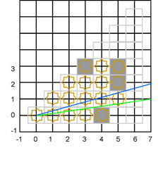
Scenario Three
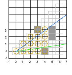
Cells (3,2) and (4,2) are unambiguously in the shadow of cell (2,1). But look carefully at column five. Even though the top vector does not pass through any part of (5,2) it does pass slightly above point (5,1) and therefore the division will round up such that (5,2) is considered visible! With this rounding algorithm you can “peek around a corner” a little bit. Visible point (5,2) is an artifact.
Even worse, consider what happens when the algorithm discovers that there is an opaque-to-transparent transition between (5,2) and (5,1). The top vector will be moved up!
That top vector is now steeper than it used to be. (Also note that if this had been the top vector when processing column four then the point (4,2) ought to have been visible.)
Obviously this situation can continue; rounding errors in later columns can continue to make the top vector steeper and steeper. (Exercise for the reader: is there a maximum slope that the top vector can attain via repeated applications of rounding error?)
We could easily put a check into the algorithm implementation to say that the top direction vector must never go from a shallower slope to a steeper slope. If we decided to use always-round-up rounding then we might do that. But it gets worse:
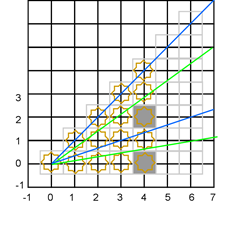
Scenario Four
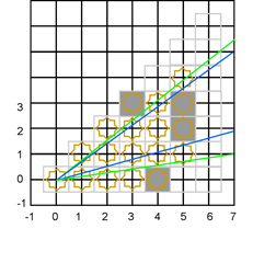
Last time I made the simplifying assumption that cell (5,4) was out of range, and therefore not visible. But suppose the radius is larger; let’s analyze this one in more detail. We’ll round up to determine the highest visible cell in the column portion bounded by these vectors, so cell (5,4) is visible. We then find transitions from visible (5,4) to opaque (5,3) and opaque (5,2) to visible (5,1) (assuming that (5,1) is the bottom cell of the range; we’ll discuss that assumption next time.) Therefore we have to divide this up into two sub-portions for column six. To compute the upper portion we keep the top vector the same and move the bottom vector up; to compute the lower portion we keep the bottom vector the same and move the top vector down. The result is this godawful mess:
The top direction vector of the upper column portion is now below the bottom vector. Yikes!
This error again allows the player to “look around corners” in a weird way, but it really is not so bad. What will happen here is that as long as the mis-ordered vectors identify the same cell as the top and bottom cell of the visible portion for a particular column, that single cell will be visible. As soon as the portion is large enough that the top and bottom cells are different, the loop that goes from top to bottom will immediately exit.
Again, we could prevent this situation by doing a check that verifies that the bottom vector is never moved to be above the top vector. However, perhaps we’d decide that this situation is sufficiently rare, and the artifact is sufficiently benign, that we’d just allow it.
Rounding up seems better than rounding down, but this still isn’t great. Hmm. What if we rounded to the nearest lattice point?
Scenario One is unchanged. We still correctly compute visibility of the entire long straight wall.
Scenario Two is unchanged. We still make the desirable “corner artifact”.
Scenario Three is improved. Cell (5,2) is not treated as visible, which is good because it is entirely in shadow. The top vector is not made more steep.
Scenario Four is unchanged. We can still end up in a situation where the top and bottom direction vectors are mis-ordered.
That’s no change in three scenarios and a great improvement in one, so this is an unambiguous win, right? Not quite.
Scenario Five
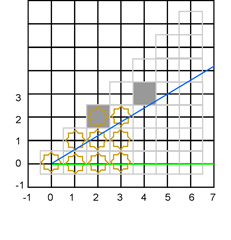
If we round to nearest then (4,3) is not visible, even though a full 30% of its lower surface has line of sight from the origin. Furthermore, by not treating this cell as visible, we fail to lower the slope of the top vector from 3/5 to 5/9, possibly allowing more cells to be visible in higher columns that ought to be shadowed by (4,3). Round-up would have treated (4,3) as the topmost cell in the region, so round-to-nearest is not an unambiguous win over round-up.
At this point it would be wise to take a step back and ask ourselves if continuing to tweak how the division rounds is the right thing to do. When you propose three different plausible calculations and they all turn out to be wrong in different ways, there might be an invalid assumption somewhere in the mix.
The invalid assumption is that y = SomeKindOfRoundingOf(x, top.Y, top.X) is correct in the first place. It is not. This calculation, no matter how you round it, is fundamentally calculating where the vector intersects the center of the column. Why is the center of the column at all relevant? It is the edges of the cell that cast shadows!
What we want to compute is “what is the highest cell in the given column that is anywhere intersected by the top direction vector?” The slope of the top direction vector is always positive; the line is always “sloping up”, so the top cell can be identified by figuring out where the vector leaves the column. What we should be doing is working out the intercept of the vector with x + 0.5, not with x.
How are we going to do that? The first thing to observe is that (x + 0.5 ) * top.Y / top.X is the same thing as (2 * x + 1) * top.Y / (2 * top.X). Now everything is in integers. Let’s work out the quotient and the remainder in integers:
int quotient = ((2 * x + 1) * top.Y) / (2 * top.X);
int remainder = ((2 * x + 1) * top.Y) % (2 * top.X);
Let’s look at a bunch of possible different possibilities. Suppose the direction vector is (5, 3), so we go five “right” for every three “up”. The interesting points are the points where the vector exits the column on the right hand side. The quotient is the black horizontal line below the interesting point. In this example the remainder is the number of tenths the interesting point is above the quotient line. (Tenths because the denominator is 5 x 2.) The numbers at the bottom of each column are the remainders
(Note that the dividend will always be an odd number and the divisor will always be an even number, and therefore the remainder will always be an odd number. Proving those assertions is left as an exercise. Hint: what possible y values can the top direction vector take on if restricted only to integers?)
So, how should we round? Consider the columns labeled 1 and 3. In those the rounded-down quotient correctly identifies the cell that the direction vector intersects. The columns labeled 7 and 9, however, have a problem; the quotient is one below the correct result; we have rounded down incorrectly. What about the column labeled 5? If the remainder is exactly the “run” value of the top direction vector then the vector passes exactly through the boundary where two cells meet; which one should be visible? Since this is the “top” bounding vector, we should round down; no area of the upper cell is visible.
So, in summary: use the rounded-down quotient as the top cell in the column if the remainder is top.X or less; otherwise, round it up by adding one to the quotient.
Does that solve our problems?
Scenario One: Good. We correctly put the whole corridor wall into the field of view.
Scenario Two: Good. We “correctly” put the invisible corner cell into the field of view.
Scenario Three: Good. Cell (5,2) is not identified as being visible, and therefore the top vector’s slope is not increased.
Scenario Four: Bad. We incorrectly identify cell (5,4) as being visible through cell (5,3), and thereby produce not only an artifact, but an “inverted” set of top and bottom vectors for the next column.
Scenario Five: Good. We make cell (4,3) visible and lower the slope of the top vector accordingly.
This algorithm is not perfect; we still make some artifacts. How might we solve the issue of scenario four?
A couple ways come to mind. One is that we could check to see if the direction vector enters the column at (5,3) and exits at (5,4). If it does then (5,4) is only the top cell if (5,3) is transparent.
Another way would be to allow cell (5,4) to be visible regardless — this might have nice properties for showing corners, even if the cell is technically an artifact — but to detect whether the new bottom vector is steeper than the old top vector and not allow the recursion.
In my actual implementation of last week I decided that solving the problem of scenario four is not worth it to me; I allow the artifacts and the inverted range. The results seem pretty decent.
As I warned you, it took me an extremely long article with nine complicated diagrams to figure out how to divide two numbers to determine the top cell. I said this was going to be excessively detailed!
Next time we’ll do the same analysis for determining the bottom cell in the column portion. Hopefully things will go a bit quicker now that we have the basic idea of how rounding produces artifacts down pat.
I hope the basic idea of the shadow casting algorithm is now clear. Let’s start to implement the thing. There are two main concerns to deal with. The easy one is “what should the interface to the computation look like?” The second is “how to implement it?” Let’s deal with the easy one first; let’s design the API.
What does the caller need to provide?
The coordinates of a central point
The radius of the field of view
Some way for the algorithm to know which cells are opaque
What does the implementation need to do for the caller?
Provide some way of telling the caller which cells are visible from the central point.
It’s that last one that is a bit tricky. The implementation could return a list of point objects that are in view. Or it could create a two-dimensional array of bools and set the bools to true if the cell is in view or false if it is not. It could mutate a caller-provided collection. And so on. We don’t know how the caller works or what it is going to do with that information. We don’t even know if it is storing that information as bools or bit flags or a list of points. It is hard to know what the right thing to do is, so we’ll punt on it. We’ll make the caller decide by making the caller pass in an Action that does the right thing for it!
public static class ShadowCaster
{
// Takes a circle in the form of a center point and radius, and a function that
// can tell whether a given cell is opaque. Calls the setFoV action on
// every cell that is both within the radius and visible from the center.
public static void ComputeFieldOfViewWithShadowCasting(
int x, int y, int radius,
Func<int, int, bool> isOpaque,
Action<int, int> setFoV)
{
// The miracle happens here
}
OK, so that’s the point of entry for the caller. What about the implementation?
I wanted my implementation to have the following characteristics:
First and foremost, the implementation should be clear and correct. It should be performant enough for small demos, but not necessarily wringing every last drop of performance out of the processor. If the code is clear and correct but not fast enough, targeted performance analysis can find the hot spot later. For debuggability, I’d like it if the code operates more or less in the same order as in the description of the algorithm I laid out. Also, the code should be DRY — Don’t Repeat Yourself. (*)
I want the implementation to not be overly concerned with vexing book-keeping details. We laid out the algorithm as one which assumed that the viewpoint was the origin and the field of view was calculated only in the zero octant; our implementation should do the same, rather than trying to keep track of details like where the viewpoint really is.
This algorithm is often implemented recursively but I wanted to avoid that, for two reasons. First, because the typical recursive implementation recurses at least once per column; one can imagine a scenario in which a long narrow tunnel hundreds of cells long blows the stack. Second, because the typical recursive implementation explores the octant in a “column depth first” manner. That is, when it must divide the visible region into multiple “portions” each with its own top and bottom direction vector, it explores each portion through to the final column; the priority is to explore each portion entirely before starting on the next. But we characterized the algorithm as a straightforward left-to-right, top-to-bottom progression of cells that explores each column entirely before starting on the next. As I said before, for both clarity and debuggability it would be nice if the implementation matched the description.
The basic idea of my implementation goes like this:
For each column, take as an input a set of cells in a column known to be either definitely in the field of view, or possibly just barely out-of-radius.
From that set, compute which cells in the next column are either definitely in the field of view or possibly just out-of-radius.
Repeat until you get to the column that is entirely outside of the field-of-view radius; you can stop there.
That’s a good high-level overview, but let’s make the action a bit more crisp:
Break each column (identified by the x-axis coordinate that defines the center of the column) down into one or more contiguous “portions” each bounded by a top and bottom direction vector.
For each portion in the current column, determine the set of portions in the subsequent column that are visible.
Add each of those subsequent portions to a work queue.
Keep on processing portions from the work queue until there are no more.
OK, that’s enough of a description to actually write some code to implement these abstractions. We can do that with two little immutable structs.
Recall that we decided to represent direction vectors as a point on the line of the vector, and that we do not care about the magnitude, only the direction. As we’ll see, the only direction vectors we need fall on lattice points, so we can use ints as the coordinates.
private struct DirectionVector
{
public int X { get; private set; }
public int Y { get; private set; }
public DirectionVector(int x, int y)
: this()
{
this.X = x;
this.Y = y;
}
}
The portion of the column we are dealing with is characterized by three facts: what is the x-coordinate of the column’s center, what is the direction vector bounding the top of the portion, and what is the direction vector bounding the bottom of the portion?
private struct ColumnPortion
{
public int X { get; private set; }
public DirectionVector BottomVector { get; private set; }
public DirectionVector TopVector { get; private set; }
public ColumnPortion(int x, DirectionVector bottom, DirectionVector top)
: this()
{
this.X = x;
this.BottomVector = bottom;
this.TopVector = top;
}
}
Now that we have these data structures we can make the main loop of the engine. Note that we are now assuming that the center point is the origin and that we are only interested in octant zero. Somehow the entry point is going to have to figure out how to deal with that requirement, but that’s a problem that we’ll solve later.
queue.Enqueue(new ColumnPortion(0, new DirectionVector(1, 0), new DirectionVector(1, 1)));
while (queue.Count != 0)
{
var current = queue.Dequeue();
if (current.X >= radius)
continue;
ComputeFoVForColumnPortion(
current.X,
current.TopVector,
current.BottomVector,
isOpaque,
setFieldOfView,
radius,
queue);
}
}
The action of the main loop is straightforward. We make a work queue. We know that all of column 0 is in the field of view and that its top and bottom vectors are the lines emanating from the origin that bound the entire octant. We put that on the work queue. We then sit in a loop taking work off the queue and processing each portion of the column. Doing so may put arbitrarily more work on the queue for the next column. Since the work queue is a queue, we guarantee that we complete one column before we start working on the next; this makes the action of the algorithm similar to that of the description of the algorithm.
The attentive reader will have noticed that we’ve already made a very interesting choice that actually fails to correctly implement the stated algorithm. If the column portion on the queue is outside of the radius of the field of view then we discard it without processing it. This guarantees that the algorithm will terminate, and also makes sure that we don’t do unnecessary work computing a column that is entirely outside of the field of view. That in of itself is fine; the interesting choice is that the comparison is
if (current.X >= radius)
and not
if (current.X > radius)
If we are asked for a field of view of radius six we do not actually make any cells in column six visible even though exactly one of them might be visible — namely, the cell at (6, 0). Every other cell in that column is more than six units away from the origin. Why make this choice?
Aesthetics. Suppose there are no obstacles, and we compute the field of view of radius six for all eight octants. The resulting field of view will look like this:
O
OOOOOOO
OOOOOOOOO
OOOOOOOOOOO
OOOOOOOOOOO
OOOOOOOOOOO
OOOOOO@OOOOOO
OOOOOOOOOOO
OOOOOOOOOOO
OOOOOOOOOOO
OOOOOOOOO
OOOOOOO
O
Which looks bizarre. The curvature of a circle by definition should appear to be the same everywhere; this makes the circle look extremely pointy at four places. The boundary of a circle should be convex everywhere; if you imagine joining the center points of all the O’s along the boundary they make for a convex hull except at eight points where the circle suddenly becomes concave. This is terribly ugly; to eliminate this ugliness we round off to an octagon by omitting the extreme column:
Much nicer. And the “error” is small, both in that it is only four points that are removed, and small in the sense that these are the four points that are the farthest-away points visible from the center; if you’re going to eliminate points, those are the most sensible ones to take away.
Today we saw that a small rounding decision can have a big impact on the aesthetics of the algorithm; next time we’ll dig into the first statement of ComputeFoVForColumnPortion and discover that subtle decisions about managing rounding errors can make a big difference in determining how the output looks to the player.
(*) Many implementations of this algorithm you find on the internet needlessly repeat all of the code eight times, once for each octant.
I’ve always loved the “roguelike” games; perhaps you’ve played some of them. Those are the games where you get a top-down view of a tile-based world, and have as much real time as you like to make a choice of action. The canonical plot is to enter a dungeon, get to the bottom, retrieve the Amulet of Yendor, and make it back out of the dungeon with it. As you might expect, the original game with these characteristics was called “Rogue“, and it has spawned many far more complex imitators. I’m particularly fond of Nethack, which I have completed twice in many, many hundreds of attempts. Hard game, Nethack.
The original Rogue had a very simplistic approach to lighting the dungeon: when you entered a lit room, you could see everything in the room regardless of whether it was behind an obstacle or not. More modern roguelike games have had increasingly more sophisticated algorithms for determining lighting that take obstacles, light intensity, and so on, into account. I was curious to see what different techniques existed for simulating realistic lighting in roguelike games, and I quickly found the collection of articles on RogueBasin on “Field of View”.
Though I really appreciate the effort that went into writing these articles and the implementations — in particular, the articles by Gordon Lipford, Björn Bergström and Henri Hakl — I must say that I found a number of them difficult to follow. There are a lot of subtleties to these algorithms, and some of these articles use common important words from geometry (like “slope”, “line” and “angle”) in unusual and inconsistent ways. When I looked at various implementations of various algorithms that people had – again, very helpfully – published, I found a lot of good stuff but also some questionable programming practices and uncommented subtle choices.
I thought what I might do then, both for my own education and as a public service, is to describe one of the algorithms in excessive detail, implement it, and describe the various factors I considered when choosing implementation techniques.
First off, before we get into the details, here’s a little Silverlight application that demonstrates what I mean. Click on the control below and then use the cursor arrow keys to move you (the “at” sign”) around. Notice that you can only see so far — about nine or ten squares in any direction — and that obstacles cast shadows. In particular, notice how shadows behave in the region that contains a lot of tightly-spaced “pillars”. Do the shadows behave realistically? While pondering that question, see if you can find the treasure and escape with it!
There was a Silverlight app here at one time!
My first ever published roguelike game is apparently pretty easy.
Ray Casting
The algorithm most people first think of when considering how to do realistic lighting is “ray casting”. That is, you imagine a circle around the player that is the limit of their light source. For each cell along the edge of the circle, imagine a ray of light emanating from the player towards the center of that cell. Work out what the first object, if any, the ray encounters along its way. All the cells that the ray passes through until the first obstacle are “visible”; the ray casting terminates at that first obstacle.
This algorithm can work, but it has a number of drawbacks. The major drawback is that if the circle is large then the number of rays that must be cast is large. Lots of rays means that the region close to the player is “visited” over and over again, which seems like it’s bad for performance. It would be nice if every cell was processed only once, or, almost as good, that every cell is processed only a small number of times.
Shadow Casting
The algorithm I’ve actually implemented here is called “shadow casting”; the basic idea of the algorithm is that rather than tracking the individual rays of light, instead we assume that everything in the circle is lit and then figure out which cells are necessarily in shadow. I’m going to start by describing the algorithm geometrically, and then we’ll see how the code implementation matches or deviates from the geometrical description.
So let’s precisely define some terms here. The world consists of a two-dimensional Euclidean plane of points. Points are represented by pairs of real numbers of the form (x,y). We use the standard geometrical convention that x increases as we move “east” and y increases as we move “north”. (*) The point (0,0) is called the “origin”.
The world contains objects that inhabit this plane. Every object is centered on a “lattice point” (x,y) where x and y are both integers, and entirely fills the square bounded by (x-0.5, y – 0.5) in the bottom left corner and (x+0.5, y+0.5) in the top right corner. That region is called the “cell” associated with the lattice point.
The “field of vision” (FoV) problem is to determine which cells are “in line of sight” from a particular point (or, in some algorithms, from any point in a given cell) when given a collection of objects that can block sight and a maximum distance.
Without loss of generality, we’re going to solve the FoV problem assuming that the “particular point” in question is the origin. As we’ll see later, we can do a simple coordinate transformation to solve the problem at other points.
Direction Vectors
The primary tool we’re going to use to solve this problem is the “direction vector”. A “vector” is like a line segment that emanates from the origin. A vector has both a magnitude and a direction, but for our purposes we will only be concerned with the direction. The direction of a (non-zero-length) vector can be described in a number of ways:
Name a point other than the origin which the vector, when extended in a straight line from the origin, would pass through; that determines the direction of the vector.
Name a point (x,y) as above; divide the y coordinate of that point by the x coordinate to obtain the “slope”. (**)
Draw a unit circle centered on the origin. Extend the vector, if necessary, to pass through the circle. Now measure the distance moving counter-clockwise from the point where the circle touches the x axis to the point where the circle touches the vector. That arc length is the angle of the vector measured in radians. Multiply by 180 / pi to get the angle in degrees.
We could use any of these methods. The disadvantage of the “slope” and “angle” methods is that in our application, slopes and angles will often be fractions that cannot be represented exactly in floating point arithmetic; it would be nice to be able to do all the arithmetic exactly. (Another disadvantage is that slopes increase to infinity as the vector angle approaches 90°, though as we’ll see, we’ll actually never be working with vectors whose slopes are larger than one or smaller than zero.) In our application it turns out that all the vectors we deal with will pass through a lattice point. We’ll therefore use the “name a point” mechanism for characterizing a direction vector.
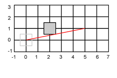
Here we have a picture illustrating the situation so far. The transparent grey box represents the cell centered on the origin. The filled-in grey box represents an object filling cell (2, 1). The red line represents a direction vector emanating from the origin and passing through (5, 1).
The Basic Idea of the Algorithm
The basic idea of the algorithm goes like this:
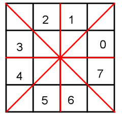
We’ve already said that without loss of generality, we’re going to solve the FoV problem assuming that the cell is the origin. Furthermore, we’re going to solve the problem only on octant zero of the plane. If you imagine direction vectors at 0°, 45°, 90°, 135°, 180°, 225°, 270° and 315° degrees, you see that those eight vectors divide the plane into eight “octants”: (***)
If we can solve the problem in octant zero then we can solve the problem in every other octant by simply reflecting the desired octant into octant zero. For example, to compute FoV in octant seven we could “reflect” all the points in octant seven through the x axis, and hey, now we’re in octant zero again.
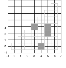
So, how are we going to solve the problem in octant zero? We will divide the cells whose centers fall into, or on the edges of this octant into columns: (****) Here we see columns zero through six; three of the columns are occupied by opaque cells. The question is, of these cells which are within six units of the origin such that an observer at the origin would have the ability to see the cell?
We’re going to go column by column, left to right. Within each column we are going to scan from top to bottom. We start with a pair of vectors. The pair of vectors represents a region of the world that is not in shadow.
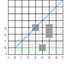
We start off with the vectors (1,0) and (1,1) because the whole of column zero is in the field of view. Remember, we are interested in the vectors only for their direction, not their magnitude, so I’m going to extend the vectors along their directions indefinitely. When processing column zero, this is the situation:
The “upper” vector is in blue and the “lower” vector is in green. The cells that fall between these vectors are the ones thus far believed to be in the field of view of the origin for this octant. We make a note that cell (0,0) in column zero is visible from column zero.
We then scan column one from top to bottom. We do not find anything that would block the view, so the vector state is unchanged after scanning column one, and every cell in column one is visible from the origin. Same for column two. However, when we come to column three we immediately find at the top of column three an opaque cell, but below it there is a transparent cell. We therefore lower the upper vector to account for the fact that the cell at (3,3) is possibly blocking the view of something in a later column.
We do not find anything else opaque in column three, so after processing column three the state of the algorithm now looks like this: (known-to-be-visible cells are marked with a sunburst.)
All of column three was in view, including the opaque cell. But now the upper vector has been lowered. When we start scanning column four, we start from the top, but the top cell in column four is now outside of the region enclosed by the vectors. It is not visible. We start scanning column four from cell (4, 3) downward. We discover that there is an opaque cell at the bottom of column four, so this time we raise the lower vector. At the end of processing column four the state of the algorithm is:
Notice something interesting: the viewable angle is getting smaller and smaller, so even though the columns are getting taller, the actual number of cells we’re scanning per column is not growing. This means that it is likely that this algorithm has better performance the more obstacles there are! That’s a nice property to have.
Now we come to the first really interesting part of the algorithm. Is cell (5,4) visible? From a strict physics perspective, clearly no portion of cell (5, 4) is visible from an observer exactly at the origin. Any possible line-of-sight vector from the origin either goes through the opaque cell at (3,3) or the opaque cell at (5,3). However, we are scanning each column from the top down; we haven’t processed cell (5, 3) yet. Another interesting question is: suppose cell (5,3) were transparent; then would cell (5,4) be visible? Its lower right corner would have line of site to the origin, but its center would not. Does that matter? Fortunately, we are saved from having to answer this question because the cell (5, 4) is out of range; we can only see for six units and (5,4) is farther away than that from the origin. However, in general we will need to consider this matter more carefully.
By similar logic, we need to decide whether cell (5,0) is visible or not. Clearly from a “physics” perspective again it is not; it is entirely blocked by cell (4, 0). There might however be implementation or gameplay reasons why we’d want to fudge things a little and allow (5,0) to be visible. We’ll come back to these points and consider them in detail when we dive into the exact implementation. For now, let’s suppose for the sake of presenting the idea of the algorithm than somehow a miracle happens and we consider cell (5, 3) to be the uppermost visible cell of column five and (5,1) to be the lowermost visible cells of column five. As we did when processing column three, we discover that there is a visible opaque cell above a visible transparent cell, and so we lower the upper vector:
And now there are no cells left that are both less than six units from the origin and have line-of-sight; we’re done. The field of view has been determined.
Let’s take a briefer look at another scenario. Suppose we have already processed a bunch of columns:
Everything in column four is visible. But what are the vectors to compute the visible cells of columns five and six? We need two sets of vectors now!
When computing the FoV of columns five and six we’ll consider both pairs of vectors as possibly containing viewable area. Naturally, if there were larger columns with many small gaps in them then we could end up generating even more vector pairs.
That’s the basic idea of the algorithm; next time we’ll try to actually implement it in C# and see what difficulties we run into.
(*) The fact that many computer display systems do not follow this convention is one of the things that makes it unnecessarily difficult to reason about code that implements these lighting systems. Some implementations assume that when given a rectangle with corners (0,0) and (1,1) the origin is the top left corner, not the bottom left corner as would be conventional geometrically. I think the best thing to do is to follow the geometrical convention, and do a transformation to the display coordinate system in code specifically tasked with making that transformation.
(**) Some implementations of this algorithm that you find on the internet define the “slope” as the negative of the “run” divided by the negative of the “rise”. Slope is more conventionally defined as the “rise” divided by the “run”, as I do here.
(***) Some implementations of this algorithm that you find on the internet define octant zero as what I here define as octant two. I think it is more consistent with general practice to number the octants counter-clockwise starting from the x-axis, just as angles are conventionally measured counter-clockwise from the x axis.
(****) Some implementations call these collections of cells “lines”, which is a bit confusing; they are not geometric lines, they are columns of cells.
First: One of the questions I get most frequently is “can you recommend some good books about learning to program better in C#?” The question is usually asked by a developer; the other day I was surprised to get that question from one of the editors of InformIT. She was kind enough to post the list on the InformIT web site, so check it out.
A lot of people really love the idea of cryptography. To computer geeks like us there is nothing cooler than the idea that computing relatively simple arithmetic on a message can enable you to communicate secretly with anyone in the world, even if there are eavesdroppers. Unfortunately, this means that there are a lot of computer people out there who are enamored with the idea of creating their own cryptosystems, or their own implementations of the cryptosystems invented by others. It also means there are a lot of software product managers who are convinced that security equals cryptography, and that their products will magically become “secure” if only there is more crypto in them.
I’ve gotten a fair number of questions over the years about how to add crypto to applications — a subject that I am actually not an expert on — and most of the time the answer is “don’t”. Many times, the question comes from a developer who, though an expert developer of applications in their line of business doesn’t “get” the basic idea of cryptography. As a public service, let me lay it out for you. The fundamental idea of modern cryptography is this:
The strength of the security of a large quantity of data — known as the “plaintext” — against discovery or modification by a motivated attacker depends upon the security of a small quantity of data — known as the “key”. (*)
That is, modern crypto is essentially a form of mechanical advantage. With a gearing system or a lever you can turn a small motion into a large motion. With a strong cryptosystem you can turn the security of a 1 KB key file into the security of a 10 MB data file. Cryptosystems do not manufacture new security, any more than a lever manufactures new motion. Cryptosystems turn the security of one thing (the key) into the security of another much larger thing (the plaintext).
It is the failure to understand that fundamental idea that underlies most of the questions I get from non-crypto experts about implementing crypto in their applications. Non-crypto experts get enamoured with the math of the cryptosystem but that is not the part that provides the security. The part that provides the security is the security of the key. The cryptosystem itself (or its implementation) might be weak or strong, but even the strongest modern cryptosystem depends fundamentally on the correct management of the keys for its security .
Before the 1970’s, all modern cryptosystems were “shared key” systems. That is, if Alice wanted to send a message to Bob over an insecure channel that had attackers attempting to either read or modify the message, then first Alice and Bob would somehow communicate a secret shared key over a secure channel. Once Alice and Bob both had the shared key, Alice could encrypt the message with the shared key, send it over the insecure channel, and Bob could decrypt it with the shared key. Bob would then have the plaintext message, but the eavesdropper would only have the encrypted message. (There are also techniques in shared-key systems whereby Bob could verify that no one tampered with the encrypted message while it was in the insecure channel.)
Clearly the security of this system depends entirely on there being a secure channel over which Alice and Bob can negotiate what their small shared key is. If they try to exchange the secret key over an insecure channel then an eavesdropper can determine what the secret key is, and it’s no longer a secret. (As we’ll see later, a more aggressive “man in the middle” can cause even more havoc.)
You might immediately wonder why Alice and Bob need to use crypto at all if a basic assumption is that they have a secure method for key exchange. Why not just use the required-to-be-secure channel for sending the unencrypted text? The point is that the secure channel might be extremely expensive, or it might be available only at certain times. For example, the “secure channel” might be that Alice and Bob meet for coffee in Seattle in their hidden underground bunker, decide on a secret key, and then Alice moves to Switzerland and Bob moves to the Cayman Islands, and they can no longer cheaply meet for coffee. But they can still communicate securely after their key exchange, even if they are no longer in the same room together.
The security of the system also depends upon them both Alice and Bob being able to keep that key a secret. If Alice or Bob reveals the key to a third party — say Eve, the eavesdropper — then Eve can discover the plaintext of every message sent over the insecure channel. Worse, if the key is discovered by Mallory — the “man in the middle” modifying the message — then she can not only discover the plaintext but can modify the plaintext, encrypt the modified message with the secret key, and send the fake message to Alice or Bob, purporting to be the other.
What about public key cryptosystems? Don’t they solve this problem? Turns out, no. Now you have four key management problems. Let me explain:
The idea of a public key cryptosystem is that there are two keys. One, the private key, is kept secret. The other, the public key, is — you guessed it — public. A message encrypted with the public key cannot be decrypted with the public key, but it can be decrypted with the private key, and vice versa. Alice and Bob both have a key pair; they do not know each other’s private keys, but they do know each other’s public keys. To send a message to Bob, Alice encrypts it with her private key(**), and then encrypts that with Bob’s public key. She sends the twice-encrypted message over the insecure channel to Bob. Bob decrypts it with his private key, and then decrypts the result with Alice’s public key. Now he knows that only he could read the message, because only he has his private key. And he knows that it was not tampered with, because only Alice’s public key could decrypt the message. Therefore the message was neither read by Eve nor tampered with by Mallory.
Like I said, we now have four key management problems whereas before we had one. Before, Alice and Bob had to securely exchange their private key and then keep it secret. Now Alice and Bob both have to keep their private keys secret. If Bob’s private key is compromised then Eve can read any message sent by Alice to Bob. And if Alice’s private key is compromised then Mallory can send a fake message to Bob purporting to come from Alice.
That’s two; what are the other two key management problems? I completely glossed over the most important part of the system! The detail that the security of the entire system rests on is that bit above where I said “but they do know each other’s public keys”. Somehow they had to securely exchange public keys. Why’s that?
Suppose Alice and Bob are sending each other their public keys. How do they do that? If they do it over an insecure channel, it does not matter if Eve can read the public keys. They are public, after all. But it matters very much if Mallory can modify the keys in transit! If Alice sends her public key to Bob over an insecure channel then Mallory can intercept the message and replace Alice’s public key with Mallory’s public key. Mallory now knows Alice’s public key, and Bob believes that Mallory is Alice! When Alice sends a message to Bob, Mallory can intercept it and replace it with a different message encrypted with Mallory’s private key and Bob’s public key. Bob decrypts the message with his private key and Mallory’s public key, believing it to be Alice’s public key, and Mallory has tricked Bob into thinking that she is Alice.
Similarly, when Bob sends his public key to Alice, Mallory can intercept it and replace it with Mallory’s public key. When Alice sends a message to Bob she encrypts it with her private key and Mallory’s public key, thinking that it is Bob’s public key. Mallory can intercept it, decode it with her private key, read the message, and re-send it along to Bob, encrypted with Bob’s real public key.
Somehow there has to be a secure channel by which public keys are exchanged. Remember, the entire point of crypto is to turn the security of a small amount of data into the security of a large amount of data. If the keys aren’t secure — either because the private keys are compromised or the public keys are not correctly associated with their real owners — then the communication is not secure at all.
This is not of theoretical concern; we have to solve this problem in real life. When you go to a web site that is going to take your credit card number, you want some assurances that first, no eavesdropper is going to be able to see that credit card number when it goes over the wire, and second, that when you send your credit card to a web site, you really are communicating with the real web site, not a fake hacker web site that looks just like it. You might not know the public key of the web site! Without a secure mechanism to obtain that public key, you might be obtaining the man-in-the-middle’s public key.
This problem is in practice solved by both the client (you) and the server (the web site) agreeing to trust a third party called the Certifying Authority, or CA. When the web site sends you the certificate containing their name and public key, the certificate is encrypted with the CA’s private key. By decrypting it with the CA’s public key, you can verify that the CA vouches for that web site actually being associated with that public key. Of course, if you do not trust the certifying authority, or the web site does not obtain certification from that certifying authority, then the key negotiation fails and the browser gives you some error message about the certificate not being verified.
But hold on a minute. Now we have yet another key management problem. The CA has to keep their private key a secret, and the CA has to somehow tell you what their public key is without being attacked by a man in the middle purporting to be the CA! We seem to have not solved the problem at all, but rather just pushed it off another level. How do we finally solve this problem once and for all? Can we use even more crypto?
Nope. This is the point where the crypto stops. (***) It has to stop somewhere; again, the point of crypto is to turn the security of a small thing into the security of a large thing; that security has to come from somewhere originally, just as the energetic motion of a lever has to come from somewhere outside the lever mechanism. The secure transmission of the CA’s public key is the piece that has to be accomplished without using any crypto. How you accomplish that is up to you; typically the operating system comes pre-installed with a list of known public keys of certifying authorities that have been verified independently by the operating system vendor. New CA “root” certificates can also be installed by your machine or network administrator. The CA roots are the organizations you trust to make security-impacting decisions on your behalf.
I seem to have strayed somewhat from my original point, but I hope I’ve made myself clear: the hard part of a secure design that uses crypto is not the math. When adding crypto to an application, the fundamental question you should be asking yourself is not “what math am I going to do on the plaintext to encrypt it?” The fundamental question is “how are my users going to generate keys, securely exchange secret keys or public keys, and keep the secret keys private?” The security of the entire system rests upon being able to leverage the secure generation and distribution of the keys into the security of the message, so solve the key management problem first.
(*) A cryptosystem is strong or weak to the extent that it delivers on this fundamental goal. If the security of the message can be compromised without the user compromising the key then the cryptosystem is weak. The goal of modern crypto is to create cryptosystems that deliver on this promise.
(**) In a realistic scenario she encrypts a hash and appends that to the message, because that is higher performance. But let’s gloss over that detail.
(***) Just to complete the sketch: the way HTTPS actually works is that a shared “session” key is securely exchanged between the client and the server. The shared key is then used to encrypt and decrypt all the messages sent between the client and the server. As we already discussed, to exchange that shared key we need a secure channel. To obtain a secure channel, the client and the server agree upon a mutually trusted CA. The server convinces the client that the agreed-upon CA vouches for the server’s public key, and so the client now has the real public key of the server. The client can then suggest a shared session key to use for the rest of the communication, and send it to the server encrypted with the server’s public key. So: the secure transmission of the shared session key relies upon (1) the secrecy of the server’s private key, (2) the secrecy of the CA’s private key, and (3) that the client and the server both have an accurate copy of the CA’s public key, obtained through some non-crypto-based secure channel. The cryptosystem leverages the secrecy of two private keys and the successful transmitting of one public key into the security of the messages transmitted in the session. If any of those keys are compromised then the whole system falls apart. (To deal with that problem, CA’s also provide the service of publishing a “revocation list” of servers that have lost control of their private keys, so that you know to not trust those guys.)
class Alpha<X>
where X : class
{}
class Bravo<T, U>
where T : class
where U : T
{
  Alpha<U> alpha;
}
This gives a compilation error stating that U cannot be used as a type argument for Alpha‘s type parameter X because U is not known to be a reference type. But surely Uis known to be a reference type because U is constrained to be T, and T is constrained to be a reference type. Is the compiler wrong?
Of course not. Bravo<object, int> is perfectly legal and gives a type argument for U which is not a reference type. All the constraint on U says is that U must inherit from T. (More specifically, it must inherit from T or be identical to T, or inherit from a type related to T by some variant conversion. Consult the specification for details.) int inherits from object, so it meets the constraint. All struct types inherit from at least two reference types, and some of them inherit from many more. Enum types inherit from System.Enum, many struct types implement interface types, and so on.
The right thing for the developer to do here is of course to add the reference type constraint to U as well.
That easily-solved problem got me thinking a bit more deeply about the issue. I think a lot of people don’t have a really solid understanding of what “inheritance” means in C#. It is really quite simple: a derived type which inherits from a base type implicitly has all inheritable members of the base type. That’s it! If a base type has a member M then a type that inherits from it has a member M as well.
Of course that’s not quite it; there are some odd corner cases. For example, a class which “inherits” from an interface must have an implementation of every member of that interface, but it could do an explicit interface implementation rather than exposing the interface’s members as its own members. This is yet another reason why I’m not thrilled that we chose the word “inherits” over “implements” to describe interface implementations. Also, certain members like destructors and constructors are not inheritable.
People sometimes ask me if private members are inherited; surely not! What would that even mean? But yes, private members are inherited, though most of the time it makes no difference because the private member cannot be accessed outside of its accessibility domain. However, if the derived class is inside the accessibility domain then it becomes clear that yes, private members are inherited:
class B
{
  private int x;
  private class D : B
  {
D inherits x from B, and since D is inside the accessibility domain of x, it can use x no problem.
I am occasionally asked “but how can a value type, like int, which is 32 bits of memory, no more, no less, possibly inherit from object? An object laid out in memory is way bigger than 32 bits; it’s got a sync block and a virtual function table and all kinds of stuff in there.” Apparently lots of people think that inheritance has something to do with how a value is laid out in memory. But how a value is laid out in memory is an implementation detail, not a contractual obligation of the inheritance relationship! When we say that int inherits from object, what we mean is that if object has a member — say, ToString — then int has that member as well. When you call ToString on something of compile-time type object, the compiler generates code which goes and looks up that method in the object’s virtual function table at runtime. When you call ToString on something of compile-time type int, the compiler knows that int is a sealed value type that overrides ToString, and generates code which calls that function directly. And when you box an int, then at runtime we do lay out an int the same way that any reference-typed object is laid out in memory.
But there is no requirement that int and object be always laid out the same in memory just because one inherits from the other; all that is required is that there be some way for the compiler to generate code that honours the inheritance relationship.
Well that was entirely predictable; as I said last time, if you ask ten developers for a definition of “type”, you get ten different answers. The comments to the previous article make for fascinating reading!
Here’s my attempt at describing what “type” means to me as a compiler writer. I want to start by considering just the question of what a type is and not confuse that with how it is used.
Fundamentally, a type in C# is a mathematical entity that obeys certain algebraic rules, just as natural numbers, complex numbers, quaternions, matrices, sets, sequences, and so on, are mathematical entities that obey certain algebraic rules.
By way of analogy, I want to digress for a moment and ask the question “what is a natural number? ” That is, what fundamentally characterizes the numbers 0, 1, 2, 3, … that we use to describe the positions of items in a sequence and the sizes of everyday collections of things?
This question has received a lot of attention over the centuries; the definitive answer that we still use today was created by Giuseppe Peano in the 19th century. Peano said that a natural number is defined as follows:
Zero is a natural number.
Every natural number has a “successor” natural number associated with it.
No natural number has zero as its successor.
Unequal natural numbers always have unequal successors.
If you start from zero, take its successor, and then take the successor of that, and so on, you will eventually encounter every natural number. (*)
Surprisingly, that’s all you need. Any mathematical entity that satisfies those postulates is usable as a natural number. (**) Notice that there’s nothing in there whatsoever about adding natural numbers together, or subtracting, multiplying, dividing, taking exponents, and so on. All of those things can be bolted on as necessary. For example, we can say that addition is defined as follows:
(n + 0) = n
(n + (successor of m)) = ((successor of n) + m)
And you’re done; you’ve got a recursive definition of addition. We can similarly define “less than”:
(n < 0) = false
(0 < (successor of m)) = true
((successor of n) < (successor of m)) = (n < m)
We can define every operation on natural numbers in this way; try defining multiplication, just for fun. (Hint: assume that you’ve already defined addition.)
We can come up with a similar “axiomatic” definition of “type”:
Object is a type
“Declared” types are types (note that int, uint, bool, string, and so on can be considered “declared” types for our purposes; the runtime “declares” them for you.)
If T is a type and n is a positive integer then “n-dimensional array of T” is also a type.
And that’s pretty much it as far as “safe” C# 1.0 is concerned. (To be as strict as the Peano axioms for natural numbers we’d want to also throw in some similar safeguards; for example, we don’t ever want to be in a situation where the type “one-dimensional array of double” has typeequality with the type “int”, just as we don’t ever want to be in a situation where the successor of a natural number is zero.)
Things get a bit more complex when we throw in generic types and pointer types, but I’m sure you can see that we could come up with a precise axiomatic description of generic types and pointer types with a little bit of work. That is, type parameter declarations are types, generic type declarations constructed with the right number of type arguments are types, and so on.
We can then start piling on algebraic operations. Just as we defined “less than” on numbers, we can define the “is a subtype of” relation on types.
T <: object is true for any type T that is not object
object <: T is false for any type T
if S <: T and T <: U then S <: U
… and so on…
Just as I do not care how numbers are “implemented” in order to manipulate them algebraically, I also do not care how types are “implemented” in order to manipulate them with the rules of type algebra. All I care about are the axioms of the system, and the rules that define the algebraic operators that I’ve made up for my own convenience.
So there you go; we have a definition of “type” that does not say anything whatsoever about “a set of values” or “a name”. A type is just an abstract mathematical entity, a bit like a number, that obeys certain defining axioms, and therefore can be manipulated algebraically by making up rules for useful operators — just like numbers can be manipulated abstractly according to algebraic rules that we make up for them.
Now that we have a sketch of an axiomatic definition of what a type is, what are we going to do with it?
Perhaps the most fundamental purposes of static type checking in a programming language like C# are to associate a type with every relevant storage location, to associate a type with every (†) relevant compile-timeexpression, and to then ensure that it is impossible for a value associated with an incompatible type to be written to or read from any storage location. A compile-time proof of runtime type safety ( ‡ ): that’s the goal.
The key word there is proof; now that we have developed an axiomatic definition of “type” we can start constructing proofs based on these axioms. The C# specification defines:
what type is associated with every compile-time expression; of course, expressions whose types cannot be determined might be program errors
what type is associated with every storage location
what constitutes an acceptable assignment from an expression of given type ( ‡‡ to a storage location of a given type
The task of the compiler writer is then to implement those three parts of the specification: associating a type with every expression, associating a type with every storage location, and then constructing a proof that the assignment is valid given the rules. If the compiler is able to construct a proof then the assignment is allowed. The tricky bit is this: the specification typically just gives the rules of the system, not a detailed algorithm describing how to construct proofs using those rules. If any proof exists then the compiler is required to find it. Conversely, if no proof exists, the compiler is required to deduce that too and produce a suitable compile-time type error.
Unfortunately, as it turns out, that’s impossible in general. A system where it is possible for every expression to be classified as either “type safe” or “type unsafe” in a finite number of logical steps is called a “decidable” system. As Gödel famously proved, natural number arithmetic as axiomatized above is undecidable; there are statements in formal arithmetic that can be neither proved nor disproved in a finite number of logical steps. Assignment type checking is also in general undecidable in programming languages with both nominal subtyping ( ‡‡ ‡ ) and generic variance. As I mentioned a while back, it turns out that it would be possible to put additional restrictions on type declarations such that nominal subtyping would become decidable, but we have not ever done this in C#. Rather, when faced with a situation that produces an infinitely long proof of type compatibility, the compiler just up and crashes with an “expression was too complex to analyze” error. I’m hoping to fix that in a hypothetical future version of the compiler, but it is not a high priority because these situations are so unrealistic.
Fortunately, situations where type analysis is impossible in general, or extremely time consuming, are rare in realistic C# programs; rare enough that we can do a reasonable job of writing a fast compiler.
Summing up: A type is an abstract mathematical entity defined by some simple axioms. The C# language has rules for associating types with compile-time expressions and storage locations, and rules for ensuring that the expression type is compatible with the storage type. The task of the compiler writer is to use those axioms and algebraic rules to construct a proof or disproof that every expression has a valid type and that every assignment obeys the assignment compatibility rules.
Though the axioms of what makes a type are pretty simple, the rules of associating types to expressions and determining assignment compatibility are exceedingly complex; that’s why the word “type” appears 5000 times in the specification. To a large extent, the C# language is defined by its type rules.
———————-
(*) I am of course oversimplifying here; more formally, the real axiom formally states that proof by induction works on natural numbers. That is: if a property is true of zero, and the property being true for a number implies the truth for its successor, then the property holds for all numbers.
(**) It is instructive to consider why the third, fourth and fifth postulates are necessary. Without the third postulate, there need only be one number: zero, which is its own successor! Without the fourth postulate we could say that there are only two numbers: the successor of zero is one, the successor of one is one. Without the fifth postulate there could be *two* zeros: “red zero” and “blue zero”. The successor of red zero is red one, the successor of blue zero is blue one, and so on. In each case, the system without the axiom satisfies the remaining four axioms, but in each case it seems very contrary to our intuition about what a “natural number” is.
(†) We fudge this in C# of course; null literals, anonymous functions and method groups are technically classified as “expressions without any type”. However, in a legal program they must occur in a context where the type of the expression can be inferred from its surrounding context.
( ‡‡ ) Again, this is fudged in a few places. For example, it is not legal to assign an expression of type int to a variable of type short, unless the expression of type int is a compile-time constant known to fit into a short.
( ‡‡ ‡ ) That is, a language where you state the base type of a newly declared type. Like “interface IFoo<T> : IBar<T>” uses nominal subtyping.






 Fabulous adventures in coding

