Before we get started, thanks for all the great comments to the previous couple of posts. I’ll be updating the algorithm to try to make even better-looking circles of light based on the comments. Like I said, there’s a lot of subtleties to these algorithms and I am just learning about them myself.

To that end, in today’s episode I am going to spend the entire prolix article analyzing a single division operation. You have been warned.

Before we begin though, some jargon. A cell which is invisible that by our physical interpretation ought to be visible, or a cell which is visible that ought to be invisible we will call an “artifact”. An “artifact” is the product of our algorithm (or some detail of its implementation) not being a sufficiently accurate model of real-world physics. Today’s article will be all about artifacts.

The actual workhorse that implements the field-of-view algorithm is this method that we mentioned last time:

private static void ComputeFoVForColumnPortion(
    int x,
    DirectionVector topVector,
    DirectionVector bottomVector,
    Func<int, int, bool> isOpaque,
    Action<int, int> setFieldOfView,
    int radius,
    Queue<ColumnPortion> queue)
{

This method has two main purposes. First, it assumes that all points in the portion of column x bounded by the top and bottom vectors are in the field of view, and marks them accordingly; some of them might be outside the radius, but the rest of them are by assumption visible from the origin. Second, it determines which portions of column x+1 are in the field of view and adds them to the work queue for later processing.

We described the algorithm as working from top to bottom of the portion of the column under consideration. Therefore the very first question we must answer is “which exactly is the top cell in the column portion, given the column number and the top direction vector?”

If the center point of a cell in column x happens to fall exactly on the top direction vector then it is pretty clear which is the top cell. Suppose for the sake of argument that’s the case. The top cell is then computed by x * topVector.Y / topVector.X. This division is exact. Proving that is an easy bit of algebra and is left as an exercise.

So perhaps we should say that even if the division is inexact, we compute the top cell by:

int topY = x * topVector.Y / topVector.X;

(Note that we’ll assume throughout that the numbers we are multiplying and dividing are small compared to the range of int, and therefore do not overflow.)

What happens if the division is inexact? We know that in C# an inexact integer division always rounds towards zero; it rounds down if necessary.

Rounding down is a bad idea because it doesn’t model the physical world well and makes for extraordinarily bad-looking gameplay. Consider this extremely common scenario:

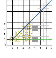
Scenario One

After processing column one we lower the slope of the top direction vector to one-third. Is point (2,1) in the field of view? It sure seems light it ought to be since its entire bottom surface is within the field of view. But if we do 2 * 1 / 3 we get zero, so no, the top cell that is visible in this column is (2, 0). We mark that as visible and continue on to column three without changing the slope. The top direction vector now intersects the center of cell (3, 1), so it and (3, 0) are visible. We lower the slope of the top vector to one-seventh, and now cell (4, 1) is not visible, again because we are rounding down. After processing all the columns shown here the state of affairs would be:

This matches neither the desired physics nor the desired gameplay; a straight corridor should not have weird “gap” artifacts. Notice also that the resulting top vector is a little bit too steep; we never considered the opaque cell in column four to be possibly shadowing anything beyond it; the rest of the world is only in the shadow of cell (3,1), not (4,1). Rounding down is clearly unacceptable.

Well. What to do, if rounding down doesn’t work? Maybe we should round up!

That solves the problem for long corridors; now what happens is cell (2,1) is determined to be visible by rounding up, so the top slope is lowered to one-fifth. Then cell (3, 1) is determined to be visible, so the slope is lowered to one-seventh. Then cell (4,1) is determined to be visible, and the slope is lowered to one-ninth.  That seems to be much better.

Moreover, we now also have the nice property that the corners of a room are visible:

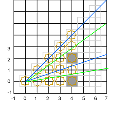
Scenario Two

Cell (5,2) will be visible, which will render nicely, particularly if “box drawing” characters are used to represent interior corners as is the case in many roguelike games. This is a desirable artifact.

But surely now we have the opposite problem; if we round up then we are potentially making cells visible that ought to be in the shadow of some opaque cell. Let’s take a look at an example of that.

Scenario Three

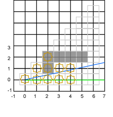
Cells (3,2) and (4,2) are unambiguously in the shadow of cell (2,1). But look carefully at column five. Even though the top vector does not pass through any part of (5,2) it does pass slightly above point (5,1) and therefore the division will round up such that (5,2) is considered visible! With this rounding algorithm you can “peek around a corner” a little bit. Visible point (5,2) is an artifact.

Even worse, consider what happens when the algorithm discovers that there is an opaque-to-transparent transition between (5,2) and (5,1). The top vector will be moved up!

That top vector is now steeper than it used to be. (Also note that if this had been the top vector when processing column four then the point (4,2) ought to have been visible.)

Obviously this situation can continue; rounding errors in later columns can continue to make the top vector steeper and steeper. (Exercise for the reader: is there a maximum slope that the top vector can attain via repeated applications of rounding error?)

We could easily put a check into the algorithm implementation to say that the top direction vector must never go from a shallower slope to a steeper slope. If we decided to use always-round-up rounding then we might do that. But it gets worse:

Scenario Four

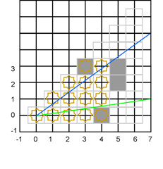
Last time I made the simplifying assumption that cell (5,4) was out of range, and therefore not visible. But suppose the radius is larger; let’s analyze this one in more detail. We’ll round up to determine the highest visible cell in the column portion bounded by these vectors, so cell (5,4) is visible. We then find transitions from visible (5,4) to opaque (5,3) and opaque (5,2) to visible (5,1) (assuming that (5,1) is the bottom cell of the range; we’ll discuss that assumption next time.) Therefore we have to divide this up into two sub-portions for column six. To compute the upper portion we keep the top vector the same and move the bottom vector up; to compute the lower portion we keep the bottom vector the same and move the top vector down. The result is this godawful mess:

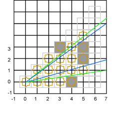
The top direction vector of the upper column portion is now below the bottom vector. Yikes!

This error again allows the player to “look around corners” in a weird way, but it really is not so bad. What will happen here is that as long as the mis-ordered vectors identify the same cell as the top and bottom cell of the visible portion for a particular column, that single cell will be visible. As soon as the portion is large enough that the top and bottom cells are different, the loop that goes from top to bottom will immediately exit.

Again, we could prevent this situation by doing a check that verifies that the bottom vector is never moved to be above the top vector. However, perhaps we’d decide that this situation is sufficiently rare, and the artifact is sufficiently benign, that we’d just allow it.

Rounding up seems better than rounding down, but this still isn’t great. Hmm. What if we rounded to the nearest lattice point?

• Scenario One is unchanged. We still correctly compute visibility of the entire long straight wall.
• Scenario Two is unchanged. We still make the desirable “corner artifact”.
• Scenario Three is improved. Cell (5,2) is not treated as visible, which is good because it is entirely in shadow. The top vector is not made more steep.
• Scenario Four is unchanged. We can still end up in a situation where the top and bottom direction vectors are mis-ordered.

That’s no change in three scenarios and a great improvement in one, so this is an unambiguous win, right? Not quite.

Scenario Five

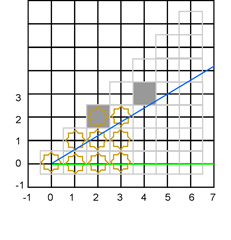
If we round to nearest then (4,3) is not visible, even though a full 30% of its lower surface has line of sight from the origin. Furthermore, by not treating this cell as visible, we fail to lower the slope of the top vector from 3/5 to 5/9, possibly allowing more cells to be visible in higher columns that ought to be shadowed by (4,3). Round-up would have treated (4,3) as the topmost cell in the region, so round-to-nearest is not an unambiguous win over round-up.

At this point it would be wise to take a step back and ask ourselves if continuing to tweak how the division rounds is the right thing to do. When you propose three different plausible calculations and they all turn out to be wrong in different ways, there might be an invalid assumption somewhere in the mix.

The invalid assumption is that y = SomeKindOfRoundingOf(x, top.Y, top.X) is correct in the first place. It is not. This calculation, no matter how you round it, is fundamentally calculating where the vector intersects the center of the column. Why is the center of the column at all relevant? It is the edges of the cell that cast shadows!

What we want to compute is “what is the highest cell in the given column that is anywhere intersected by the top direction vector?” The slope of the top direction vector is always positive; the line is always “sloping up”, so the top cell can be identified by figuring out where the vector leaves the column. What we should be doing is working out the intercept of the vector with x + 0.5, not with x.

How are we going to do that? The first thing to observe is that (x + 0.5 ) * top.Y / top.X is the same thing as (2 * x + 1) * top.Y / (2 * top.X). Now everything is in integers. Let’s work out the quotient and the remainder in integers:

int quotient = ((2 * x + 1) * top.Y) / (2 * top.X);
int remainder = ((2 * x + 1) * top.Y) % (2 * top.X);

Let’s look at a bunch of possible different possibilities. Suppose the direction vector is (5, 3), so we go five “right” for every three “up”. The interesting points are the points where the vector exits the column on the right hand side. The quotient is the black horizontal line below the interesting point. In this example the remainder is the number of tenths the interesting point is above the quotient line. (Tenths because the denominator is 5 x 2.) The numbers at the bottom of each column are the remainders

(Note that the dividend will always be an odd number and the divisor will always be an even number, and therefore the remainder will always be an odd number. Proving those assertions is left as an exercise. Hint: what possible y values can the top direction vector take on if restricted only to integers?)

So, how should we round? Consider the columns labeled 1 and 3. In those the rounded-down quotient correctly identifies the cell that the direction vector intersects. The columns labeled 7 and 9, however, have a problem; the quotient is one below the correct result; we have rounded down incorrectly. What about the column labeled 5? If the remainder is exactly the “run” value of the top direction vector then the vector passes exactly through the boundary where two cells meet; which one should be visible? Since this is the “top” bounding vector, we should round down; no area of the upper cell is visible.

So, in summary: use the rounded-down quotient as the top cell in the column if the remainder is top.X or less; otherwise, round it up by adding one to the quotient.

Does that solve our problems?

• Scenario One: Good. We correctly put the whole corridor wall into the field of view.
• Scenario Two: Good. We “correctly” put the invisible corner cell into the field of view.
• Scenario Three: Good. Cell (5,2) is not identified as being visible, and therefore the top vector’s slope is not increased.
• Scenario Four: Bad. We incorrectly identify cell (5,4) as being visible through cell (5,3), and thereby produce not only an artifact, but an “inverted” set of top and bottom vectors for the next column.
• Scenario Five: Good. We make cell (4,3) visible and lower the slope of the top vector accordingly.

This algorithm is not perfect; we still make some artifacts. How might we solve the issue of scenario four?

A couple ways come to mind. One is that we could check to see if the direction vector enters the column at (5,3) and exits at (5,4). If it does then (5,4) is only the top cell if (5,3) is transparent.

Another way would be to allow cell (5,4) to be visible regardless — this might have nice properties for showing corners, even if the cell is technically an artifact — but to detect whether the new bottom vector is steeper than the old top vector and not allow the recursion.

In my actual implementation of last week I decided that solving the problem of scenario four is not worth it to me; I allow the artifacts and the inverted range. The results seem pretty decent.

As I warned you, it took me an extremely long article with nine complicated diagrams to figure out how to divide two numbers to determine the top cell. I said this was going to be excessively detailed!

Next time we’ll do the same analysis for determining the bottom cell in the column portion. Hopefully things will go a bit quicker now that we have the basic idea of how rounding produces artifacts down pat.

I hope the basic idea of the shadow casting algorithm is now clear. Let’s start to implement the thing. There are two main concerns to deal with. The easy one is “what should the interface to the computation look like?” The second is “how to implement it?” Let’s deal with the easy one first; let’s design the API.

What does the caller need to provide?

• The coordinates of a central point
• The radius of the field of view
• Some way for the algorithm to know which cells are opaque

What does the implementation need to do for the caller?

• Provide some way of telling the caller which cells are visible from the central point.

It’s that last one that is a bit tricky. The implementation could return a list of point objects that are in view. Or it could create a two-dimensional array of bools and set the bools to true if the cell is in view or false if it is not. It could mutate a caller-provided collection. And so on. We don’t know how the caller works or what it is going to do with that information. We don’t even know if it is storing that information as bools or bit flags or a list of points. It is hard to know what the right thing to do is, so we’ll punt on it. We’ll make the caller decide by making the caller pass in an Action that does the right thing for it!

public static class ShadowCaster
{
    // Takes a circle in the form of a center point and radius, and a function that
    // can tell whether a given cell is opaque. Calls the setFoV action on
    // every cell that is both within the radius and visible from the center.
    public static void ComputeFieldOfViewWithShadowCasting(
        int x, int y, int radius,
        Func<int, int, bool> isOpaque,
        Action<int, int> setFoV)
    {
        // The miracle happens here
    }

OK, so that’s the point of entry for the caller. What about the implementation?

I wanted my implementation to have the following characteristics:

First and foremost, the implementation should be clear and correct. It should be performant enough for small demos, but not necessarily wringing every last drop of performance out of the processor. If the code is clear and correct but not fast enough, targeted performance analysis can find the hot spot later. For debuggability, I’d like it if the code operates more or less in the same order as in the description of the algorithm I laid out. Also, the code should be DRY — Don’t Repeat Yourself. (*)

I want the implementation to not be overly concerned with vexing book-keeping details. We laid out the algorithm as one which assumed that the viewpoint was the origin and the field of view was calculated only in the zero octant; our implementation should do the same, rather than trying to keep track of details like where the viewpoint really is.

This algorithm is often implemented recursively but I wanted to avoid that, for two reasons. First, because the typical recursive implementation recurses at least once per column; one can imagine a scenario in which a long narrow tunnel hundreds of cells long blows the stack. Second, because the typical recursive implementation explores the octant in a “column depth first” manner. That is, when it must divide the visible region into multiple “portions” each with its own top and bottom direction vector, it explores each portion through to the final column; the priority is to explore each portion entirely before starting on the next. But we characterized the algorithm as a straightforward left-to-right, top-to-bottom progression of cells that explores each column entirely before starting on the next. As I said before, for both clarity and debuggability it would be nice if the implementation matched the description.

The basic idea of my implementation goes like this:

• For each column, take as an input a set of cells in a column known to be either definitely in the field of view, or possibly just barely out-of-radius.
• From that set, compute which cells in the next column are either definitely in the field of view or possibly just out-of-radius.
• Repeat until you get to the column that is entirely outside of the field-of-view radius; you can stop there.

That’s a good high-level overview, but let’s make the action a bit more crisp:

• Break each column (identified by the x-axis coordinate that defines the center of the column) down into one or more contiguous “portions” each bounded by a top and bottom direction vector.
• For each portion in the current column, determine the set of portions in the subsequent column that are visible.
• Add each of those subsequent portions to a work queue.
• Keep on processing portions from the work queue until there are no more.

OK, that’s enough of a description to actually write some code to implement these abstractions. We can do that with two little immutable structs.

Recall that we decided to represent direction vectors as a point on the line of the vector, and that we do not care about the magnitude, only the direction. As we’ll see, the only direction vectors we need fall on lattice points, so we can use ints as the coordinates.

private struct DirectionVector
{
    public int X { get; private set; }
    public int Y { get; private set; }
    public DirectionVector(int x, int y)
        : this()
    {
        this.X = x;
        this.Y = y;
    }
}

The portion of the column we are dealing with is characterized by three facts: what is the x-coordinate of the column’s center, what is the direction vector bounding the top of the portion, and what is the direction vector bounding the bottom of the portion?

private struct ColumnPortion
{
    public int X { get; private set; }
    public DirectionVector BottomVector { get; private set; }
    public DirectionVector TopVector { get; private set; }
    public ColumnPortion(int x, DirectionVector bottom, DirectionVector top)
        : this()
    {
        this.X = x;
        this.BottomVector = bottom;
        this.TopVector = top;
    }
}

Now that we have these data structures we can make the main loop of the engine. Note that we are now assuming that the center point is the origin and that we are only interested in octant zero. Somehow the entry point is going to have to figure out how to deal with that requirement, but that’s a problem that we’ll solve later.

private static void ComputeFieldOfViewInOctantZero(
    Func<int, int, bool> isOpaque,
    Action<int, int> setFieldOfView,
    int radius)
{
    var queue = new Queue<ColumnPortion>();
    queue.Enqueue(new ColumnPortion(0, new DirectionVector(1, 0), new DirectionVector(1, 1)));
    while (queue.Count != 0)
    {
        var current = queue.Dequeue();
        if (current.X >= radius)
            continue;
        ComputeFoVForColumnPortion(
            current.X,
            current.TopVector,
            current.BottomVector,
            isOpaque,
            setFieldOfView,
            radius,
            queue);
    }
}

The action of the main loop is straightforward. We make a work queue. We know that all of column 0 is in the field of view and that its top and bottom vectors are the lines emanating from the origin that bound the entire octant. We put that on the work queue. We then sit in a loop taking work off the queue and processing each portion of the column. Doing so may put arbitrarily more work on the queue for the next column. Since the work queue is a queue, we guarantee that we complete one column before we start working on the next; this makes the action of the algorithm similar to that of the description of the algorithm.

The attentive reader will have noticed that we’ve already made a very interesting choice that actually fails to correctly implement the stated algorithm. If the column portion on the queue is outside of the radius of the field of view then we discard it without processing it. This guarantees that the algorithm will terminate, and also makes sure that we don’t do unnecessary work computing a column that is entirely outside of the field of view. That in of itself is fine; the interesting choice is that the comparison is

if (current.X >= radius)

and not

if (current.X > radius)

If we are asked for a field of view of radius six we do not actually make any cells in column six visible even though exactly one of them might be visible — namely, the cell at (6, 0). Every other cell in that column is more than six units away from the origin. Why make this choice?

Aesthetics. Suppose there are no obstacles, and we compute the field of view of radius six for all eight octants. The resulting field of view will look like this:

       O      
    OOOOOOO
   OOOOOOOOO
  OOOOOOOOOOO
  OOOOOOOOOOO
  OOOOOOOOOOO
 OOOOOO@OOOOOO
  OOOOOOOOOOO
  OOOOOOOOOOO
  OOOOOOOOOOO
   OOOOOOOOO
    OOOOOOO
       O      

Which looks bizarre. The curvature of a circle by definition should appear to be the same everywhere; this makes the circle look extremely pointy at four places. The boundary of a circle should be convex everywhere; if you imagine joining the center points of all the O’s along the boundary they make for a convex hull except at eight points where the circle suddenly becomes concave. This is terribly ugly; to eliminate this ugliness we round off to an octagon by omitting the extreme column:

    OOOOOOO
   OOOOOOOOO
  OOOOOOOOOOO
  OOOOOOOOOOO
  OOOOOOOOOOO
  OOOOO@OOOOO
  OOOOOOOOOOO
  OOOOOOOOOOO
  OOOOOOOOOOO
   OOOOOOOOO
    OOOOOOO

Much nicer. And the “error” is small, both in that it is only four points that are removed, and small in the sense that these are the four points that are the farthest-away points visible from the center; if you’re going to eliminate points, those are the most sensible ones to take away.

Today we saw that a small rounding decision can have a big impact on the aesthetics of the algorithm; next time we’ll dig into the first statement of ComputeFoVForColumnPortion and discover that subtle decisions about managing rounding errors can make a big difference in determining how the output looks to the player.

(*) Many implementations of this algorithm you find on the internet needlessly repeat all of the code eight times, once for each octant.

I’ve always loved the “roguelike” games; perhaps you’ve played some of them. Those are the games where you get a top-down view of a tile-based world, and have as much real time as you like to make a choice of action. The canonical plot is to enter a dungeon, get to the bottom, retrieve the Amulet of Yendor, and make it back out of the dungeon with it. As you might expect, the original game with these characteristics was called “Rogue“, and it has spawned many far more complex imitators. I’m particularly fond of Nethack, which I have completed twice in many, many hundreds of attempts. Hard game, Nethack.

The original Rogue had a very simplistic approach to lighting the dungeon: when you entered a lit room, you could see everything in the room regardless of whether it was behind an obstacle or not. More modern roguelike games have had increasingly more sophisticated algorithms for determining lighting that take obstacles, light intensity, and so on, into account. I was curious to see what different techniques existed for simulating realistic lighting in roguelike games, and I quickly found the collection of articles on RogueBasin on “Field of View”.

Though I really appreciate the effort that went into writing these articles and the implementations — in particular, the articles by Gordon Lipford, Björn Bergström and Henri Hakl — I must say that I found a number of them difficult to follow. There are a lot of subtleties to these algorithms, and some of these articles use common important words from geometry (like “slope”, “line” and “angle”) in unusual and inconsistent ways. When I looked at various implementations of various algorithms that people had – again, very helpfully – published, I found a lot of good stuff but also some questionable programming practices and uncommented subtle choices.

I thought what I might do then, both for my own education and as a public service, is to describe one of the algorithms in excessive detail, implement it, and describe the various factors I considered when choosing implementation techniques.

First off, before we get into the details, here’s a little Silverlight application that demonstrates what I mean. Click on the control below and then use the cursor arrow keys to move you (the “at” sign”) around. Notice that you can only see so far — about nine or ten squares in any direction — and that obstacles cast shadows. In particular, notice how shadows behave in the region that contains a lot of tightly-spaced “pillars”. Do the shadows behave realistically? While pondering that question, see if you can find the treasure and escape with it!

There was a Silverlight app here at one time!

My first ever published roguelike game is apparently pretty easy.

Ray Casting

The algorithm most people first think of when considering how to do realistic lighting is “ray casting”. That is, you imagine a circle around the player that is the limit of their light source. For each cell along the edge of the circle, imagine a ray of light emanating from the player towards the center of that cell. Work out what the first object, if any, the ray encounters along its way. All the cells that the ray passes through until the first obstacle are “visible”; the ray casting terminates at that first obstacle.

This algorithm can work, but it has a number of drawbacks. The major drawback is that if the circle is large then the number of rays that must be cast is large. Lots of rays means that the region close to the player is “visited” over and over again, which seems like it’s bad for performance. It would be nice if every cell was processed only once, or, almost as good, that every cell is processed only a small number of times.

Shadow Casting

The algorithm I’ve actually implemented here is called “shadow casting”; the basic idea of the algorithm is that rather than tracking the individual rays of light, instead we assume that everything in the circle is lit and then figure out which cells are necessarily in shadow. I’m going to start by describing the algorithm geometrically, and then we’ll see how the code implementation matches or deviates from the geometrical description.

So let’s precisely define some terms here. The world consists of a two-dimensional Euclidean plane of points. Points are represented by pairs of real numbers of the form (x,y). We use the standard geometrical convention that x increases as we move “east” and y increases as we move “north”. (*) The point (0,0) is called the “origin”.

The world contains objects that inhabit this plane. Every object is centered on a “lattice point” (x,y) where x and y are both integers, and entirely fills the square bounded by (x-0.5, y – 0.5) in the bottom left corner and (x+0.5, y+0.5) in the top right corner. That region is called the “cell” associated with the lattice point.

The “field of vision” (FoV) problem is to determine which cells are “in line of sight” from a particular point (or, in some algorithms, from any point in a given cell) when given a collection of objects that can block sight and a maximum distance.

Without loss of generality, we’re going to solve the FoV problem assuming that the “particular point” in question is the origin. As we’ll see later, we can do a simple coordinate transformation to solve the problem at other points.

Direction Vectors

The primary tool we’re going to use to solve this problem is the “direction vector”. A “vector” is like a line segment that emanates from the origin. A vector has both a magnitude and a direction, but for our purposes we will only be concerned with the direction. The direction of a (non-zero-length) vector can be described in a number of ways:

• Name a point other than the origin which the vector, when extended in a straight line from the origin, would pass through; that determines the direction of the vector.
• Name a point (x,y) as above; divide the y coordinate of that point by the x coordinate to obtain the “slope”.  (**)
• Draw a unit circle centered on the origin. Extend the vector, if necessary, to pass through the circle. Now measure the distance moving counter-clockwise from the point where the circle touches the x axis to the point where the circle touches the vector. That arc length is the angle of the vector measured in radians. Multiply by 180 / pi to get the angle in degrees.

We could use any of these methods. The disadvantage of the “slope” and “angle” methods is that in our application, slopes and angles will often be fractions that cannot be represented exactly in floating point arithmetic; it would be nice to be able to do all the arithmetic exactly. (Another disadvantage is that slopes increase to infinity as the vector angle approaches 90°, though as we’ll see, we’ll actually never be working with vectors whose slopes are larger than one or smaller than zero.) In our application it turns out that all the vectors we deal with will pass through a lattice point. We’ll therefore use the “name a point” mechanism for characterizing a direction vector.

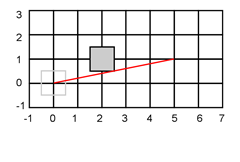
Here we have a picture illustrating the situation so far. The transparent grey box represents the cell centered on the origin. The filled-in grey box represents an object filling cell (2, 1). The red line represents a direction vector emanating from the origin and passing through (5, 1).

The Basic Idea of the Algorithm

The basic idea of the algorithm goes like this:

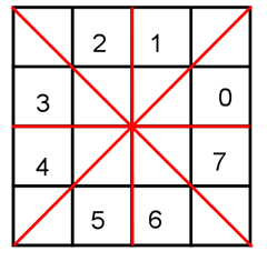
We’ve already said that without loss of generality, we’re going to solve the FoV problem assuming that the cell is the origin. Furthermore, we’re going to solve the problem only on octant zero of the plane. If you imagine direction vectors at 0°, 45°, 90°, 135°, 180°, 225°, 270° and 315° degrees, you see that those eight vectors divide the plane into eight “octants”: (***)

If we can solve the problem in octant zero then we can solve the problem in every other octant by simply reflecting the desired octant into octant zero. For example, to compute FoV in octant seven we could “reflect” all the points in octant seven through the x axis, and hey, now we’re in octant zero again.

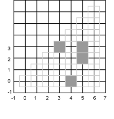
So, how are we going to solve the problem in octant zero? We will divide the cells whose centers fall into, or on the edges of this octant into columns: (****) Here we see columns zero through six; three of the columns are occupied by opaque cells. The question is, of these cells which are within six units of the origin such that an observer at the origin would have the ability to see the cell?

We’re going to go column by column, left to right. Within each column we are going to scan from top to bottom. We start with a pair of vectors. The pair of vectors represents a region of the world that is not in shadow.

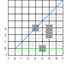
We start off with the vectors (1,0) and (1,1) because the whole of column zero is in the field of view. Remember, we are interested in the vectors only for their direction, not their magnitude, so I’m going to extend the vectors along their directions indefinitely. When processing column zero, this is the situation:

The “upper” vector is in blue and the “lower” vector is in green. The cells that fall between these vectors are the ones thus far believed to be in the field of view of the origin for this octant. We make a note that cell (0,0) in column zero is visible from column zero.

We then scan column one from top to bottom. We do not find anything that would block the view, so the vector state is unchanged after scanning column one, and every cell in column one is visible from the origin. Same for column two. However, when we come to column three we immediately find at the top of column three an opaque cell, but below it there is a transparent cell. We therefore lower the upper vector to account for the fact that the cell at (3,3) is possibly blocking the view of something in a later column.

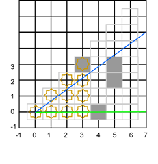
We do not find anything else opaque in column three, so after processing column three the state of the algorithm now looks like this: (known-to-be-visible cells are marked with a sunburst.)

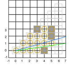
All of column three was in view, including the opaque cell. But now the upper vector has been lowered. When we start scanning column four, we start from the top, but the top cell in column four is now outside of the region enclosed by the vectors. It is not visible. We start scanning column four from cell (4, 3) downward. We discover that there is an opaque cell at the bottom of column four, so this time we raise the lower vector. At the end of processing column four the state of the algorithm is:

Notice something interesting: the viewable angle is getting smaller and smaller, so even though the columns are getting taller, the actual number of cells we’re scanning per column is not growing. This means that it is likely that this algorithm has better performance the more obstacles there are! That’s a nice property to have.

Now we come to the first really interesting part of the algorithm. Is cell (5,4) visible? From a strict physics perspective, clearly no portion of cell (5, 4) is visible from an observer exactly at the origin. Any possible line-of-sight vector from the origin either goes through the opaque cell at (3,3) or the opaque cell at (5,3). However, we are scanning each column from the top down; we haven’t processed cell (5, 3) yet. Another interesting question is: suppose cell (5,3) were transparent; then would cell (5,4) be visible? Its lower right corner would have line of site to the origin, but its center would not. Does that matter? Fortunately, we are saved from having to answer this question because the cell (5, 4) is out of range; we can only see for six units and (5,4) is farther away than that from the origin. However, in general we will need to consider this matter more carefully.

By similar logic, we need to decide whether cell (5,0) is visible or not. Clearly from a “physics” perspective again it is not; it is entirely blocked by cell (4, 0). There might however be implementation or gameplay reasons why we’d want to fudge things a little and allow (5,0) to be visible. We’ll come back to these points and consider them in detail when we dive into the exact implementation. For now, let’s suppose for the sake of presenting the idea of the algorithm than somehow a miracle happens and we consider cell (5, 3) to be the uppermost visible cell of column five and (5,1) to be the lowermost visible cells of column five. As we did when processing column three, we discover that there is a visible opaque cell above a visible transparent cell, and so we lower the upper vector:

And now there are no cells left that are both less than six units from the origin and have line-of-sight; we’re done. The field of view has been determined.

Let’s take a briefer look at another scenario. Suppose we have already processed a bunch of columns:

Everything in column four is visible. But what are the vectors to compute the visible cells of columns five and six? We need two sets of vectors now!

When computing the FoV of columns five and six we’ll consider both pairs of vectors as possibly containing viewable area. Naturally, if there were larger columns with many small gaps in them then we could end up generating even more vector pairs.

That’s the basic idea of the algorithm; next time we’ll try to actually implement it in C# and see what difficulties we run into.

(*) The fact that many computer display systems do not follow this convention is one of the things that makes it unnecessarily difficult to reason about code that implements these lighting systems. Some implementations assume that when given a rectangle with corners (0,0) and (1,1) the origin is the top left corner, not the bottom left corner as would be conventional geometrically. I think the best thing to do is to follow the geometrical convention, and do a transformation to the display coordinate system in code specifically tasked with making that transformation.

(**) Some implementations of this algorithm that you find on the internet define the “slope” as the negative of the “run” divided by the negative of the “rise”. Slope is more conventionally defined as the “rise” divided by the “run”, as I do here.

(***) Some implementations of this algorithm that you find on the internet define octant zero as what I here define as octant two. I think it is more consistent with general practice to number the octants counter-clockwise starting from the x-axis, just as angles are conventionally measured counter-clockwise from the x axis.

(****) Some implementations call these collections of cells “lines”, which is a bit confusing; they are not geometric lines, they are columns of cells.