Happy St. Valentine’s Day all. To solve the Smullyan retrograde chess puzzle posted yesterday, the first question to ask is “is the black king actually in check, or not?” In a great many retro problems the first task is to determine who is to move, and knowing that one or the other side is in check is the easiest way to do that.

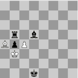
Suppose the answer is “black is not in check”. In that case there is only one place that the white king can be:

Great. Is this the answer? No. Because now white is in check. Twice. You can’t end a move in check. Therefore black just moved one of the pieces on the board in order to deliver that double check. Which one? It certainly was not the black king. But there is nowhere that the black rook or black bishop could have moved from such that white was not already in check by the other black piece! Since white did not end a move in check, it is impossible for the white king to be on B3.

Therefore the black king is in check after all. So it is black’s move. Some white piece now on the board must have moved in order to deliver that check. Which piece was it? There are only two: the white bishop and the white king. Suppose it was the bishop. Now we have the same problem again: where did the white bishop come from to deliver the check, such that black was not already in check? Nowhere, that’s where.

Therefore: black is in check. The check was a discovered check caused by the white king moving away from B3. There are only two squares that the white king can move to from B3 such that the white king is not moving into check.

Therefore: black is in check, the check was delivered by moving the white king from B3 to either A3 or C3.

Hold on a minute! Didn’t we just argue previously that the white king could not possibly have been on B3? No. We just argued that the white king could not be on B3 with the board as it is at present because there is no piece that could have delivered the double check. But the white king could have been on B3 on a board in the past with an additional black piece on it, a piece that was just captured by white, and it was that piece which delivered the seemingly-impossible double check.

So: at some point in the past the white king was on B3. Black made a move of some piece that ended on either A3 or C3, which double-checked white. White responded by taking that piece and giving a discovered check to black.

What now-taken black piece could possibly deliver that double check by moving to A3 or C3? There is only one possibility, but to see what it is we’ll need to go back a few moves.

Here’s a possible board position a few moves ago; black is to move:

It’s not required that the board have looked like this, but it is possible. Retro enthusiasts refer to this as an “unlocked” position. That is, there is no obvious impediment to legally getting from the starting position to this board position, and there are many ways to do so. From the unlocked position we then have the only possible sequence of moves that ends in the position given in the statement of the puzzle:

Black takes the knight and calls check:

White blocks the check by moving the pawn up two spaces:

Black delivers the “impossible” double check by capturing en passant:

And white captures the pawn and calls check:

…leaving the white king on C3.

There is no way to get a black piece that reveals the double check to A3, so this is the only possible solution. Can white force a draw? Who cares! Retros are about figuring out the past, not about what the outcome of the game will be.

If you like this sort of puzzle — and believe me, they get a lot more complicated than that! — Smullyan’s two books on the subject are both delightful. And if you do, a word of advice: pawns can capture en passant, pawns don’t have to promote to a queen, and just because pieces are on their starting squares doesn’t mean they’ve never moved!

It’s not going to happen in my lifetime!

Thus logician, philosopher and puzzle-constructor Raymond Smullyan, who died last week at the age of 97.

I started reading Smullyan when I was a teenager; I don’t remember whether I read This Book Needs No Title (about philosophy) or What Is The Name Of This Book? (puzzles) first, but whichever it was started a lifetime of enjoyment of both. His philosophy was decidedly playful. In one of his books he dispenses with the question “Does a dog have the Buddha-nature?” with Of course a dog has the Buddha-nature! You just have to look at some dogs to know that.

His puzzles were deceptively simple and quickly ended up being disguised versions of some very difficult topics in first order logic, combinatory logic, Boolean logic, and so on. Though he was most famous for his “Island of Knights and Knaves” puzzles, where knights can only tell the truth an knaves can only lie, he produced a great many puzzles on other topics. To Mock A Mockingbird, in which combinators are thinly disguised as singing birds, is a particular favourite; it changed my understanding of the fundamentals of computer programming.

Among my favourites of all his puzzles though were his two books of absolutely delightful retrograde chess puzzles. Most chess puzzles consider the future: from this position, what should white play next to ensure a mate? Retro puzzles are not concerned with the future, but rather the past; what had to happen in the game in order to arrive at this position?

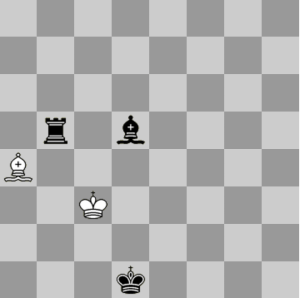
Here’s my favourite Smullyan retro, which was on the cover of my copy of Chess Mysteries of the Arabian Nights:

The white king has been removed from the board; your task is to deduce where it goes. There is only one square where the white king can be such that the position is possible to produce in a legal game of chess. (Note that I said legal, and not sensible!)

Leave your thoughts in the comments and I’ll give the answer later this week.

Last time we discussed the syntax for logical deductions that is common in academia: facts above, deductions below, a line between them. We discussed the tautology rule and the instance rule. Today: more rules.

       A ⊢ e:σ   
GEN:  ------------ ( α not free in A )
       A ⊢ e:∀ασ   

This is the “generic” rule: if you have some fact about an expression, then that fact is also true when quantified over all types. For example, if we know that A ⊢ e:int→int then we also know that we can make up a type variable α, and no matter what value we give the type variable, the expression is still of that type.

Exercise: Do you see why α must not be free? Suppose α is free in A; can you find an example of how the GEN rule produces an invalid conclusion if we were to allow this?

Now, you might say that it is obvious that if something is true, then it is also true even when we give any old value to a type variable that is not even involved. And yes, that’s obvious. It’s good that it is obvious! All these rules should be obviously correct.

What I just said was a bit of an “intuition pump”, because it is actually a bit subtle. Do you see why? Just because α is not free in A does not imply that α is not free in σ! So why is it legal to make this quantification over a variable free in σ only if it is not free in A? Ponder that briefly.

If after pondering it was not clear, don’t worry. It is a lot easier to understand these subtleties by looking at a realistic example, which we will do next time on FAIC.

In our next rule we have two facts above the line, which we have not yet seen:

       A ⊢ e:τ' → τ     A ⊢ e':τ'   
COMB: ----------------------------
       A ⊢ (e e'):τ

If we have a function from τ' to τ, and an expression of type τ', then the expression “pass the value to the function” is of type τ.

Just like in C#: if we have a function F that takes a string and returns an int, and e is an expression of type string, then F(e) is an expression of type int. Easy peasy.

If you think we need to have at least one rule for every possible kind of expression in Exp, you’re right! Fortunately there are only four kinds of expressions: identifiers, function calls, lambdas, and let expressions. We’ve already seen the first two, so it should be no surprise that the next rule is for lambdas.

This rule is a little more complicated:

       Ax ∪ { x:τ' } ⊢ e:τ
ABS:  ---------------------
       A ⊢ (λx.e):τ' → τ

Let’s sort this one out carefully.

Suppose we have a set of assumptions A that might or might not contain a judgment for identifier x. If it does, remove it. To that, add a judgment that says that x is of type τ'. And suppose from that set of assumptions we can deduce that expression e is of type τ.

That implies that from assumptions A, we can deduce that λx.e is a function from τ' to τ.

Why do we need to say Ax ∪ { x:τ' } instead of simply A ∪ { x:τ' }? Because we said at the beginning of this chapter that all sets of assumptions would contain at most one judgment for any identifier. But A ∪ { x:τ' } might contain two judgments for x, if A already contains a judgment for x.

Leaving aside the mechanisms of adding and removing judgments from a set of assumptions, I hope the rule is sensible. If knowing that x is of type τ' allows us to deduce that e is of type τ, then λx.e can be used anywhere we need a function from τ' to τ.

Notice that it does not matter whether A contains a judgment for x or not. If it does not, fine. If it does, then who cares? λx.e defines a new variable x that shadows any existing x in the environment.

We’ve seen rules for identifiers, function applications and lambdas. There is only one rule left, which describes how typing works for let expressions. Again, it takes two facts and produces a third.

       A ⊢ e:σ      Ax ∪ { x:σ } ⊢ e':τ
LET:  -----------------------------------
       A ⊢ (let x = e in e'):τ

This is very similar to the rule for lambdas. If e is of type scheme σ, and identifier x being of type scheme σ implies that e' is of type τ, then the type of the corresponding let expression is τ. Again, we need to do a little scut work to make sure that the identifier x is treated properly, but I hope the rule is clear.

These are the only rules of the deductive system. Next time we’ll go through an example of how to use the rules to start with nothing, and from that deduce some facts about identity functions.

All right, so far we’ve mostly been talking about jargon and background information. Now we’re actually going to get into the meat of the thing here. What we want is (1) a formal definition of what logical steps we are justified in using to determine what the type scheme of an expression is, when evaluated in a particular environment, and (2) an algorithm that produces a valid sequence of logical steps that ends in a type scheme for the expression.

How are we going to do that? First things first:

5 Type inference

From now on we shall assume that A contains at most one assumption
about each identifier x. Ax stands for removing any assumption about
x from A. 

That notation is a bit vexing, but I hope it is clear.

For assumptions A, expression e and type-scheme σ we write

                          A ⊢ e:σ

if this instance may be derived from the following inference rules:

Note that this is a single turnstile. Last time we used the double turnstile to mean “from a collection of typed identifiers A, we can logically deduce that an expression e has type scheme σ“. It appears that we mean the same thing by the single turnstile, but does it?

The subtle difference is “may be derived from the following inference rules”. The single turnstile means that we actually could produce a valid sequence of particular logical rules that get us to the type judgment.

But we’re getting ahead of ourselves.

I started this series because I get the question quite frequently “I tried to read this paper and I couldn’t understand the notation”. In particular, people who have no experience with the standard notation for logical deductions have a bad reaction to this notation, but really it is very straightforward. The syntax is:

       KNOWN FACTS
RULE: ------------ ( ADDITIONAL NOTES )
       DEDUCTIONS 

So, stuff you know already goes on top. The name of the deduction rule goes on the left. The deduction that this rule allows you to make goes below the line, and any additional notes about the rule go in parens beside it.

The deductions of course are themselves just facts, so we can put a line below the deductions, and make even more deductions, and so on.

In our particular deductive system, all facts and deductions will be of the form A ⊢ e:σ where again, A is a set of identifiers with types, e is an expression, and σ is a type scheme. Remember, the turnstile means “there exists a sequence of logical deductions that justifies this typing judgment”.

We call a sequence of logical deductions of this form a “derivation” of the result.

Let’s start with the easiest rule; a rule so easy you might think it isn’t necessary:

TAUT: ---------- ( x:σ ∈ A )
       A ⊢ x:σ

A “tautology” is a statement that is necessarily true by its form. “All X that are Y are Y” is a true statement no matter what we substitute for X and Y.

This rule has no facts at all above the line; tautologies are necessarily true irrespective of any particular facts. The notes on the side say that for this rule to apply, identifier x must have type scheme σ in assumptions A. Given that, we logically deduce that, surprise, from assumptions A we can deduce that the expression x is an expression of type σ.

So why do we need this rule? Because remember what the single turnstile means. The single turnstile means that we can deduce the type scheme of an identifier by producing a derivation: a sequence of logical deductions drawn from a specific set of rules. It’s not enough to say that obviously, if an assumption is true then it is true. We have to have a rule that says that so that we can use that rule in a valid sequence of rules.

Let’s look at a very slightly harder one.

       A ⊢ e:σ   
INST: ---------- ( σ > σ' )
       A ⊢ e:σ'

The “instance” rule is: if we can logically deduce from assumptions A that e is of type σ, then we can also logically deduce from assumptions A that e is of a smaller type σ'.

For example, suppose we already know that A ⊢ x:∀α(α → α). Then with this rule we can deduce further that A ⊢ x:(int → int). If we have enough evidence to deduce that x is a function from α to α for any type α then we have enough evidence to deduce that it a function from integers to integers.

This might seem a bit weird to you. Isn’t this backwards?

If in C# we deduced that x was of type Mammal, we would not consider that to be evidence for a deduction that it was of a smaller type, Giraffe. We’d consider it to be of a larger type, Animal. However, there’s another way to think of it: in C# if we deduced that x was of type Mammal, we would know that any Giraffe was a valid value for x, but not necessarily any Animal. That’s the kind of inference we’re doing here.

Next time we’ll look at some more of the rules of this deductive system.

All right, we are getting through section four of this paper. Today: what is an “environment”?

Now let Env = Id → V be the domain of environments η. 

Just to be clear, this is not a function in the Exp language. This is a formal description of part of the runtime engine of the Exp language. Basically we are saying here that an “environment” is simply the part of the runtime of an implementation of the language that takes identifiers and maps them onto their values. And that just as we’ll use σ for type schemes and α for type variables, we’ll use η for environments.

You’re so accustomed to using environments that they are like the air you breathe; you don’t even think about it. When you’re writing a program in some language and you say x = y + z;, you’re saying “obtain the values associated with identifiers y and z from the environment, add them, and modify the environment so that next time we ask, x has that value”. We can characterize the accesses to y and z as the environment being a function that takes “y” or “z” and returns their values. We can characterize the assignment to x as being the construction of a new environment based on the previous environment.

The semantic function ε : Exp → Env → V is given in [5]. 

Again this is not an function in the Exp language; this is again a formalization of the runtime engine.

Remember that in our notation, a function of two arguments is notated as a function of one argument that returns a function of one argument. So what we’re saying here is that the “semantic function” is a function that takes an expression and an environment and produces a value.

Again, this is making formal the basic operation of a runtime. The runtime has a bunch of expressions and the values of all the variables, and it evaluates the expressions in the context of the environment.

Using it, we wish to attach meaning to assertions of the form 

                           A ⊨ e:σ

where e ∈ Exp and A is a set of assumptions of the form x:σ, x∈Id.

This right here is the mission statement of this paper.

The double-turnstile means “the thing on the right is a logical consequence of the thing on the left”.

What we’re saying here is: we have (on the left) a set of judgments (called “assumptions” here) where all the expressions are identifiers. Say:

x:int
square:int → int
identity:∀β(β → β)

We have on the right an arbitrary expression with a typing judgement, say

λy.identity (square x) : ∀β(β → int)

I hope you agree that if we assume that x is an int, square is a function from int to int, and identity is an identity function, that the lambda given is a function that takes any type and returns an int. The assumptions on the left are sufficient to deduce that the judgment on the right is correct (if the assumptions are correct, of course).

The goal of this paper is to provide an algorithm which, given the facts on the left and the expression on the right, deduces the type schema on the right in a manner that allows us to confidently say that yes, we have sufficient evidence on the left to make this judgment on the right.

(Aside: is it possible to have a function with type scheme ∀β(β → β) that is not an identity function? Ponder this!)

If the assertion is closed, i.e. if A and σ contain no free type
variables, then the sentence is said to hold iff, for every 
environment η, whenever η ⟦x⟧:σ', for each member x:σ' of A,
it follows that ε ⟦e⟧ η:σ. 

OK, we’ve got some jargon and some notation here used without introduction.

First of all, “the assertion” and “the sentence” are being used interchangeably here. We are “asserting” that the assumptions about typed identifiers on the left are sufficient evidence to deduce the type of the expression on the right.

Second, remember when we abused the Exp function notation to say that an environment was a function Id → V? You would think then that we would continue to abuse that notation and say that given an environment η and an identifier x we would say that the value of x was η x. And is what we do, but to call out that x is being used here as an identifier rather than standing in for a value, we “quote” it with funny brackets. So the value of identifier x in environment η is notated η ⟦x⟧.

Similarly for the semantic function ε. It takes two things: an expression e and an environment η, and to emphasize that the expression is an expression of the Exp language, we bracket it as well. So ε ⟦e⟧ η is “the value of expression e when evaluated in environment η”.

So what the heck is this jargon-filled paragraph actually saying? We have a bunch of identifiers with types on one side, and the statement that this implies that expression on the other side has a particular type. The paragraph is saying that this means: choose any possible environment that has those identifiers having some values of the given types. No matter what environment you chose, evaluating the expression in that environment gives a value that matches the expression’s type.

That might be too abstract still. In our example:

x:int, square:int → int, identity:∀β(β → β) ⊨ 
  λy.identity (square x) : ∀β(β → int)

We’re saying that no matter what integer we choose for x, no matter what function from int to int “square” really is, and no matter what function matching its type scheme “identity” really is, we know that evaluating the expression on the right will produce a function from something to int. There is never any combination of values for the environment that would cause that expression to evaluate to something else.

Further, an assertion holds iff all its closed instances hold.

That’s maybe not so clear but fortunately there is an example in the paper:

Thus, to verify the assertion

                x:α, f: ∀β(β → β) ⊨ (f x): α

it is enough to verify it for every monotype μ in place of α.
This example illustrates that free type variables in an assertion
are implicitly quantified over the whole assertion, while explicit
quantification in a type scheme has restricted scope.

What we’re getting at here is that this is not the same as saying

                x:∀α α, f: ∀β(β → β) ⊨ (f x): α

Because that scopes the alpha to just the type of x, but we want that alpha to be still “in scope” on the right hand side of the double turnstile. Basically it is saying that the assertion is logically:

              ∀α  ( x:α, f: ∀β(β → β) ⊨ (f x): α  )

All right, that gets us through section four! The last paragraph in section four lays out what is going to happen in the rest of the paper:

The remainder of this paper proceeds as follows. First we present
an inference system for inferring valid assertions. Next we present 
an algorithm W for computing a type scheme for any expression, under
assumptions A. We then show that W is sound, in the sense that any 
type-scheme it derives is derivable in the inference system. Finally
we show that W is complete, in the sense that any derivable 
type-scheme is an instance of that computed by W.

Next time: A notation for making chains of logical inferences, and another kind of turnstile.

All right, finally we are getting to typing judgments, which are the bread and butter of type inference algorithms. We said in the previous episode that the values that are manipulated by a program written in Exp are either values of primitive types, or functions from one value to another, and that this set of values is called V:

To each monotype μ corresponds a subset V , as detailed in [5];
if v∈V is in the subset for μ we write v:μ.

Recall that a monotype is a type with no “generic” type arguments. So for instance, the monotype int has values that are all possible integers. The monotype int → int has values like “the function that takes an integer and doubles it”. This syntax simply means that the value on the left of the colon is an instance of the monotype on the right.

Further we write v:τ if v:μ for every monotype instance μ of τ, 
and we write  v:σ if v:τ for every τ which is a generic instance
of σ.

Let’s consider an example. Suppose we have the identity function λx.x and the type scheme ∀β(β → β). We could make an instance of that type scheme, say int → int. Plainly λx.x is a function that takes ints and returns ints. In fact, for any instance of that type scheme, the identity function fits the bill. So we say that λx.x:∀β(β → β).

Note that if there were even a single instance of the scheme that did not match the function, then we could not make the judgment that the function is a member of that type scheme. For example, suppose we have a function square that takes an int and returns its square. We cannot say that square:∀β(β → β) because square is not a member of, say, (int → int) → (int → int).

Next time: what is an “environment”?

So far we’ve gotten through the introduction, the grammar of the Exp language, the grammar of the type description language, and what it means to make substitutions in type schemes. For the next few episodes we’ll consider the semantics of the Exp language.

Having the grammar of the language is enough to be able to parse it, but ultimately computer programs are intended to be executed. Programs manipulate values, and so we should be able to say formally what the rules are for values and how different program elements compute them.

4 Semantics

The semantic domain V for Exp is a complete partial order 
satisfying the following equations up to isomorphism, where 
Bi is a cpo corresponding to primitive type ιi :

V = B0 + B1 + ... + F + W (disjoint sum)
F = V → V (function space)
W = {·} (error element)

HOLY GOODNESS that is a lot of jargon with no explanation.

I’m not going to go into too much detail here as formal semantic analysis using domain theory is not my strong suit. But we can unpack some of this jargon.

First off, by “semantic domain V” we pretty much mean “what are all the possible values that a variable can have?” This might not be as straightforward as you think! Consider C#:

class C<T> 
{
  int x;
  T y;
}

It’s pretty clear that the values of variable x can be any of the four billion possible ints. But what are the possible values of y? T is, from the perspective of the compiler, a perfectly legal type for y. We can now come to two incompatible conclusions. First: T can be any type, so y can have any value, including, say, 123. Second: there are no values of type T — please, try to find a running program that has a T stored in y! — so since y is of type T, there can be no values for y.

Plainly at most one of those statements can be true. The second conclusion is unsound but it is tricky to try to figure out where exactly the reasoning goes wrong.

Anyways, my point is that in a language with generics we need to be careful to describe exactly what are the possible values are that can be manipulated by the program. The “semantic domain” that we’re calling “V” here is the set of all values that can be manipulated by the Exp language.

But we say more than just that it is a set; we say that it is a “complete partial order”. What on earth is a cpo, and why do we care?

Long-time readers of this blog already know what a “total ordering” is. It’s a bunch of things, plus a relation on them that takes any two things A and B, and decides consistently whether A is larger than, smaller than, or equal to B. Total orders are necessary for sorting algorithms to work properly. A total order has all kinds of restrictions — things equal to the same are equal to each other, if A is smaller than B and B is smaller than C then A is smaller than C, A and B are never both smaller than each other, and so on. But the easiest way to think about a total order is that given any two elements, they are either equal, or one is bigger than the other.

A partial order relaxes this requirement. In a partial order, given any two elements they are equal, or one is bigger than the other, or they are unordered with respect to each other. “Unordered” and “equal” are very different!

Consider assignment compatibility in C# for example. We can make a partial order on types based on assignment compatibility.

An expression of type int is assignable to a variable of type long, so int is “less than” long. Similarly int is “less than” object. A string is assignable to object, so string is “less than” object. But ints and strings are not assignable to each other, and they certainly are not equal! They are neither bigger, nor smaller, nor equal to each other as far as the “assignment compatibility” relationship is concerned. Assignment compatibility is a partial order.

A set that comes with a partial order is called a “poset”.

A “complete” partial order is a partial order with an additional property which would be somewhat tedious for me to define, so I’m going to skip it. In fact, all of this is a bit of a digression. There are technical reasons why the study of programming language value domains needs complete partial orders. Recall that we mentioned fixed-point analysis as it applied to recursive functions a while back. Suffice to say, the mathematics of analyzing recursive functions, function application, and so on, requires that there be a partial order.

So what are we really saying here? We’re saying that the values that can be manipulated by an Exp program are:

• Any value of one of the “primitive” types
• A function that takes a value and returns a value
• A value representing “this program is an error”.

Frankly it is not 100% clear to me why we need the error element. It is never mentioned again in the paper! Anyone who has more background in domain theory who wants to clue me in here, please leave a comment.

All right, we have come to the not entirely surprising conclusion that the values manipulated in a functional language are primitive values and functions of one parameter.

Next time: typing judgments!

We take a break from a detailed exegesis of a 40-year-old paper for a brief political message.

Freakonomics did a poll to come up with a slogan for this country, and the winner was America: Our Worst Critics Prefer To Stay. I can get behind that. I’ve avoided criticizing my hosts for twenty years, and that ends now.

Yesterday I stood in a room with 42 people from 25 countries on five continents; they all put in the considerable time and effort it takes to become American citizens. Unlike the vast majority of Americans, they chose to be here. And anyone who tells you that they are in any way whatsoever not “real Americans” is selling something that I don’t buy.

Next time: back to type inference and formal semantics!

Last time we saw how we can make a substitution for a free variable to produce an instance of a type scheme. This time we’ll look at a much more powerful form of substitution.

By contrast a type-scheme σ = ∀α1...αm τ has a "generic instance"
σ' = ∀β1...βn τ' if τ' = [τi/αi]τ for some types τ1,...,τm and 
the βj are not free in σ.

This definitely needs an example.

Suppose we have the identity function λx.x. Its type scheme is ∀α α → α. Now we might want to perform a substitution here of int for α. But we’ve only defined substitution on free variables, and we need to make a substitution on bound variables, to eliminate the bound variable entirely.

This mechanism of “generic instantiation” says: a type scheme consists of zero or more quantifiers and a type. Take just the type and perform a substitution on it, and then put as many quantifiers as you like before the substituted type, provided that the new quantifiers are not turning free variables into bound variables.

Let’s try it. Extract the type from the type scheme: α → α. We perform our substitution [int/α] on that type to get int → int. And then we put zero or more quantifiers on top of that. Let’s put zero quantifiers on top of it. So we have the original type scheme ∀α α → α — that is, for all α, there’s a function from α to α. Now we want a specific generic instance of that, and it is int → int.

This is in a sense the sort of generic instantiation that you’re used to from C#. Notice that we’ve eliminated not just the type variable, but the quantifier on top of the type scheme.

Now let’s look at a more complicated example.

Suppose we have some type scheme for some function, let’s say ∀β∀γ β → γ. And let’s suppose we pass that thing to the identity function. The type scheme of the identity function is ∀α α → α: the quantifier says that this works for any α we care to name, as long as the type provided for α is a type, not a type scheme; remember, so far we’ve only described type substitution by saying that we’re going to replace a free variable with a type, but what we have is a type scheme with two bound type variables: ∀β∀γ β → γ.

How do we deal with this? We’ll do our generic instantiation process again. We have type schemes ∀α α → α and ∀β∀γ β → γ. Take just the type of the first without the quantifiers: α → α. Now make the substitution with the type of the second without the quantifiers: [β → γ / α] to get the type (β → γ) → (β → γ). Then slap a couple of quantifiers on top of that: ∀β∀γ (β → γ) → (β → γ).

We’ve produced an entirely new type scheme, but clearly this type scheme has the same “fundamental structure” as the type scheme for the identity function, even though this type scheme does not have the type variable of the original scheme, or even the same number of type variables; it’s got one more.

Why did we have to say that all of the introduced type variables must be “not free”? Well, let’s see what happens if we violate that constraint. Suppose we have type scheme ∀α β → α. Clearly β is free.

We extract the type: β → α. We perform a substitution [int/α] to get β → int. And then we put a quantifier on top: ∀β β → int. But that turns β from a free variable into a bound variable, so this is not a generic instance of a type scheme with a free variable β. Thus when creating generic instances we are restricted to introduce quantifiers only on non-free variables.

In this case we shall write σ > σ'. 

Conceptually this is pretty straightforward. Given two type schemes, possibly one is a generic instance of the other. If a schema σ’ is a generic instance of a scheme σ then we say that σ’ is smaller than σ. This should make some sense given our examples so far. If you think of schemes as patterns that can be matched, the pattern ∀α α → α is way more general than the pattern int → int, so we say that the latter is “smaller” — less general — than the former.

It is slightly problematic that the authors chose the “greater than” symbol instead of, say, the “greater than or equal” symbol. Why? Well consider ∀α α → α and ∀β β → β. It should not be hard to see that both of these are generic instances of each other, and therefore both are “smaller” than the other, which is silly. Plainly they are equally general!

Note that instantiation acts on free variables, while generic
instantiation acts on bound variables.

This line should now be clear.

 
It follows that σ > σ' implies S σ > S σ'.

Let’s look at a quick example just to make sure that’s clear. Suppose we have σ = ∀α α → β and σ' = int → β. Clearly σ > σ’. If we now make the substitution of string for β in both, then we have ∀α α → string which is still more general than int → string; clearly the greater-than relationship is preserved by substitution of free variables.

And that’s it for section 3! Next time, we’ll look at the formal semantics of the Exp language.

Last time we learned what is meant by “free” and “bound” variables both in the context of the Exp language and the type scheme language. So, substitutions:

If S is a substitution of types for type variables, often written
[τ1/α1, ... ,τn/αn] or [τi/αi] and σ is a type-scheme, then S σ 
is the type-scheme obtained by replacing each free occurrence of 
αi in σ by τi, renaming the generic variables of σ if necessary.

OK, syntactic concerns first. A substitution is written as a bracketed list of pairs, where the first element of the pair is a type (possibly a type variable, but definitely not a type scheme!) and the second is a type variable. We can think of a substitution as a function that takes a type scheme and produces a new type scheme, so (possibly confusingly) we use the same notation as we do for applying a function to an argument in the Exp language.

Let’s look at an example. Suppose we have the type scheme σ = ∀α α → (β → β), and the substitution S = [int/β]. β is free in σ, so S σ is ∀α α → (int → int).

Remember that we said last time that the free type variables were essentially type variables whose values were going to be provided by an outer context. Substitution of types for free variables is essentially a mechanism by which we can supply the value of the type variable.

Why “renaming the generic variables of σ if necessary”? Well suppose we had σ as before but the substitution S = [α/β] and we intended that α to be a different (that is, free) α than the (bound) α in σ. We cannot in this case say that S σ is ∀α α → (α → α) because now every α is bound, which is not what we want. But we can say, hey, we’ll just trivially rename the bound α to γ and now the result of the substitution is ∀γ γ → (α → α) and all is well.

Then S σ is called an "instance" of σ;

Notice that since S σ is itself a type scheme, we are saying that “instance of” is a relation on type schemes: given any two type schemes, we should be able to tell if one is an instance of another, by checking to see if there is any substitution on free variables of one that produces the other, modulo renaming of bound variables.

the notions of substitution and instance extend naturally 
to larger syntactic constructs containing type-schemes.

In later episodes we’re going to have things that contain some number of type schemes, and we want to be able to say “apply this substitution to all of them” and produce a collection of instance type schemes.

Next time: we’ve seen that we can substitute any type for a free variable to get an instance of a schema. But this is insufficiently powerful; we need to be able to make substitutions on bound variables as well, eliminating the bound variable. Next time we’ll see how to do that.