Last time on FAIC we went through a loose, hand-wavy definition of what it means to have a “weighted” continuous distribution: our weights are now doubles, and given by a Probability Distribution Function; the probability of a sample coming from any particular range is the area under the curve of that range, divided by the total area under the function. (Which need not be 1.0.)

A central question of the rest of this series will be this problem: suppose we have a delegate that implements a non-normalized PDF; can we implement Sample() such that the samples conform to the distribution?

The short answer is: in general, no.

A delegate from double to double that is defined over the entire range of doubles has well over a billion billion possible inputs and outputs. Consider for example the function that has a high-probability lump in the neighbourhood of -12345.678 and another one at 271828.18 and is zero everywhere else; if you really know nothing about the function, how would you know to look there?

We need to know something about the PDF in order to implement Sample().

The long answer is: if we can make a few assumptions then sometimes we can do a pretty good job.

---

Aside: As I’ve mentioned before in this series: if we know the quantile function associated with the PDF then we can very easily sample from the distribution. We just sample from a standard continuous uniform distribution, call the quantile function with the sampled value, and the value returned is our sample. Let’s assume that we do not know the quantile function of our PDF.

---

Let’s look at an example. Suppose I have this weight function:

double Mixture(double x) =>
  Exp(–x * x) + Exp((1.0 – x) * (x – 1.0) * 10.0);

If we graph that out, it looks like this:

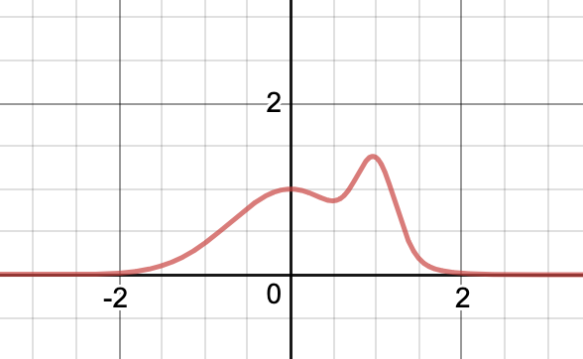
I called it “mixture” because it is the sum of two (non-normalized) normal distributions. This is a valid non-normalized PDF: it’s a pure function from all doubles to a non-negative double and it has finite area under the curve.

How can we implement a Sample() method such that the histogram looks like this?

---

Exercise: Recall that I used a special technique to implement sampling from a normal distribution. You can use a variation on that technique to efficiently sample from a mixture of normal distributions; can you see how to do so? See if you can implement it.

However, the point of this exercise is: what if we did not know that there was a trick to sampling from this distribution? Can we sample from it anyways?

---

The technique I’m going to describe today is, once more, rejection sampling. The idea is straightforward; to make this technique work we need to find a weighted “helper” distribution that has this property:

The weight function of the helper distribution is always greater than or equal to the weight function we are trying to sample from.

Now, remember, the weight function need not be “scaled” so that the area under the curve is 1.0. This means that we can multiply any weight function by a positive constant, and the distribution associated with the multiplied weight function is the same. That means that we can weaken our requirement:

There exists a constant factor such that the weight function of the helper distribution multiplied by the factor is always greater than or equal to the weight function we are trying to sample from.

This will probably be more clear with an example.

Let’s take the standard normal distribution as our helper. We already know how to sample from it, and we know it’s weight function. But it just so happens that there exists a constant — seven — such that multiplying the constant factor by the helper’s weight function dominates our desired distribution:

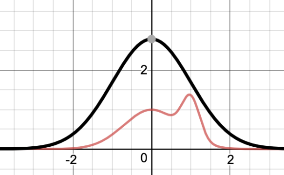
Again, we’re going to throw some darts and hope they land below the red curve.

• The black curve is the weight function of the helper — the standard normal distribution — multiplied by seven.
• We know how to sample from that distribution.
• Doing so gives us an x coordinate for our dart, distributed according to the height of the black curve; the chosen coordinate is more likely to be in a higher region of any particular width than a lower region of the same width.
• We’ll then pick a random y coordinate between the x axis and the black curve.
• Now we have a point that is definitely below the black line, and might be below the red line.
• If it is not below the red line, reject the sample and try again.
• If it is below the red line, the x coordinate is the sample.

Let’s implement it!

Before we do, once again I’m going to implement a Bernoulli “flip” operation, this time as the class:

sealed class Flip<T> : IWeightedDistribution<T>
{
  public static IWeightedDistribution<T> Distribution(
    T heads, T tails, double p)

You know how this goes; I will skip writing out all that boilerplate code. We take values for “heads” and “tails”, and the probability (from 0 to 1) of getting heads. See the github repository for the source code if you care.

I’m also going to implement this obvious helper:

static IWeightedDistribution<bool> BooleanBernoulli(double p) =>
  Flip<bool>.Distribution(true, false, p);

All right. How are we going to implement rejection sampling? I always begin by reasoning about what we want, and what we have. By assumption we have a target weight function, a helper distribution whose weight function “dominates” the given function when multiplied, and the multiplication factor. The code practically writes itself:

public class Rejection<T> : IWeightedDistribution<T>
{
  public static IWeightedDistribution<T> Distribution(
      Func<T, double> weight,
      IWeightedDistribution<T> helper,
      double factor = 1.0) =>
    new Rejection<T>(weight, dominating, factor);

I’ll skip the rest of the boilerplate. The weight function is just:

public double Weight(T t) => weight(t);

The interesting step is, as usual, in the sampling.

Rather than choosing a random number for the y coordinate directly, instead we’ll just decide whether or not to accept or reject the sample based on a Bernoulli flip where the likelihood of success is the fraction of the weight consumed by the target weight function; if it is not clear to you why that works, give it some thought.

public T Sample()
{
  while(true)
  {
    T t = this.helper.Sample();
    double hw = this.helper.Weight(t) * this.factor;
    double w = this.weight(t);
    if (BooleanBernoulli(w / hw).Sample())
      return t; 
  }
}

All right, let’s take it for a spin:

var r = Rejection<double>.Distribution(
  Mixture, Normal.Standard, 7.0);
Console.WriteLine(r.Histogram(–2.0, 2.0));

And sure enough, the histogram looks exactly as we would wish:

                             **         
                            ***         
                            ***         
                           *****        
                           *****        
                 ******   ******        
                ****************        
               *****************        
              *******************       
             ********************       
            *********************       
            *********************       
           ***********************      
          ************************      
         *************************      
        ***************************     
      *****************************     
    *********************************   
----------------------------------------

How efficient was rejection sampling in this case? Actually, pretty good. As you can see from the graph, the total area under the black curve is about three times the total area under the red curve, so on average we end up rejecting two samples for every one we accept. Not great, but certainly not terrible.

Could we improve that? Sure. You’ll notice that the standard normal distribution times seven is not a great fit. We could shift the mean 0.5 to the right, and if we do that then we can reduce the multiplier to 4:

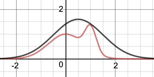
That is a far better fit, and if we sampled from this distribution instead, we’d reject a relatively small fraction of all the samples.

---

Exercise: Try implementing it that way and see if you get the same histogram.

---

Once again we’ve managed to implement Sample() by rejection sampling; once again, what are the pros and cons of this technique?

• Pro: it’s conceptually very straightforward. We’re just throwing darts and rejecting the darts that do not fall in the desired area. The darts that do fall in the desired area have the desired property: that samples from a given area arrive in proportion to that area’s size.
• Con: It is by no means obvious how to find a tight-fitting helper distribution that we can sample such that the helper weight function is always bigger than the target weight function. What distribution should we use? How do we find the constant multiplication factor?

The rejection sampling method works best when we have the target weight function ahead of time so that we can graph it out and an expert can make a good decision about what the helper distribution should be. It works poorly when the weight function arrives at runtime, which, unfortunately, is often the case.

---

Next time on FAIC: We’ll look at a completely different technique for sampling from an arbitrary PDF that requires less “expert choice” of a helper distribution.