Last time on FAIC I gave a hand-wavy intuitive explanation for why it is that lifting a function on doubles to duals gives us “automatic differentiation” on that function — provided of course that the original function is well-behaved to begin with. I’m not going to give a more formal proof of that fact; today rather I thought I’d do a brief post about multivariate calculus, which is not as hard as it sounds. (In sharp contrast to the next step, partial differential equations, which are much harder than they sound; I see that Professor Siv, as we called him, is still at UW and I hope is still cheerfully making undergraduates sweat.)

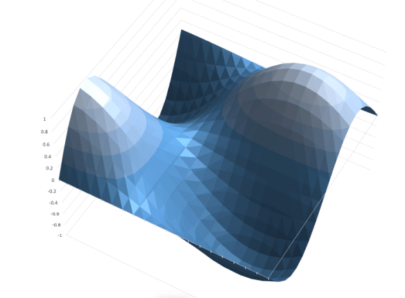
We understand that the derivative of an analytic function f(x) that takes a real and produces a real is the function f'(x) that gives the slope of f(x) at each point. But suppose we have a function that takes two reals and produces a real. Maybe f(x, y) = cos(x/5) sin(y/3). Here, I’ll graph that function from (0, 0) to (20, 20):

We could implement this in C# easily enough:

static ℝ Compute2(ℝ x, ℝ y) => Math.Cos(x / 5.0) * Math.Sin(y / 3.0);

That’s a pretty straightforward analytic function of two variables, but we’re programmers; we can think of two-variable functions as a one-variable factory that produces one-variable functions. (This technique is called currying, after the logician Haskell Curry.)

static Func<ℝ, ℝ> Compute2FromX(ℝ x) => (ℝ y) =>
  Math.Cos(x / 5.0) * Math.Sin(y / 3.0);

That is, given a value for x, we get back a function f(y), and now we are back in the world of single-variable real-to-real functions. We could then take the derivative of this thing with respect to y and find the slope “in the y direction” at a given (x, y) point.

Similarly we could go in the other direction:

static Func<ℝ, ℝ> Compute2FromY(ℝ y) => (ℝ x) =>
  Math.Cos(x / 5.0) * Math.Sin(y / 3.0);

And now given a “fixed” y coordinate we can find the corresponding function in x, and compute the slope “in the x direction”.

In wacky calculus notation, we’d say that ∂f(x, y)/∂x is the two-variable function that restricts f(x, y) to a specific y and computes the slope of that one-variable function in the x direction. Similarly ∂f(x, y)/∂y is the function that restricts f(x, y) to a specific x and computes the slope of that one-variable function in the y direction.

You probably see how we could compute the partial derivatives of a two-variable, real-valued analytic function using our Dual type; just curry the two-variable function into two one-variable functions, change all of the “doubles” to “Duals” in the “returned” function, and provide dualized implementations of sine and cosine.

But… do we actually need to do the currying step? It turns out no! We do need implementations of sine and cosine; as we discussed last time, they are:

public static ⅅ Cos(ⅅ x) =>
  new ⅅ(Math.Cos(x.r), –Math.Sin(x.r) * x.ε);
public static ⅅ Sin(ⅅ x) =>
  new ⅅ(Math.Sin(x.r), Math.Cos(x.r) * x.ε);

Easy peasy. We can now write our computation in non-curried, dualized form:

static ⅅ Compute2(ⅅ x, ⅅ y) => ⅅ.Cos(x / 5.0) * ⅅ.Sin(y / 3.0);

Now suppose we are interested in the x-direction slope and the y-direction slope at (13, 12), which is part of the way up the slope of the right hand “hill” in the graph:

Console.WriteLine(Compute2(13 + ⅅ.EpsilonOne, 12));
Console.WriteLine(Compute2(13, 12 + ⅅ.EpsilonOne));

We do the computation twice, and tell the compute engine to vary one-epsilon in the x direction the first time, and not at all in the y direction. The second time, we vary by one-epsilon in the y direction but not at all in the x direction. The output is:


0.648495546750919+0.0780265449058288ε
0.648495546750919+0.186699955809795ε


Which gives us that the slope in the x direction is about 0.078, and the slope in the y direction is about 0.187. So for the cost of computing the function twice, we can get the derivatives in both directions. Moreover, if we wanted to compute the slope in some other direction than “parallel to the x axis” or “parallel to the y axis”, perhaps you can see how we’d do that.

But we’ve actually gotten something even a bit more interesting and useful here: we’ve computed the gradient!

The gradient of a multivariate function like this one is the direction you’d have to walk to gain altitude the fastest. That is, if you are standing at point (13, 12) on that graph, and you walk 0.078 steps in the x direction for every 0.187 steps in the y direction, you’ll be heading in the “steepest” direction, which is the direction likely to get you to the top of the mountain the fastest:

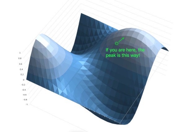
And of course if you walk in the “negative of the gradient” direction, you’re heading “downslope” as fast as possible.

Notice that heading in the “upslope” or “downslope” direction does not necessarily move you directly towards the nearest peak, valley or saddle; it heads you in the direction that is gaining or losing altitude the fastest. If you do not know exactly where the peaks and valleys are, that’s your best guess of the right direction to go.

I hope it is clear that there is no reason why this should be limited to functions of two variables, even though it is hard to visualize higher-dimensional functions! We can have a real-valued function of any number of variables, take the partial derivatives of each, and find the gradient that points us in the “steepest” direction.

Why is this useful? Well, imagine you have some very complicated but smooth multivariate function that represents, say, the cost of a particular operation which you would like to minimize. We might make an informed guess via some heuristic that a particular point is near a “cost valley”, and then compute the gradient at that point; this gives us a hint as to the direction of the nearest valley, and we can then try another, even more informed guess until we find a place where all the gradients are very small.  Or, equivalently, we might have a “benefit function” that we are trying to maximize, and we need a hint as to what direction the nearby peaks are. These techniques are in general called “gradient descent” and “gradient ascent” methods and they are quite useful in practice for finding local minima and maxima.

The point is: as long as the function you are computing is computed only by adding, subtracting, multiplying, and dividing doubles, or using double-valued library functions whose derivatives you know, you can “lift” the function to duals with only a minor code change, and then you get the derivative of that function computed exactly, for a very small additional cost per computation. That covers a lot of functions where it might not be at all obvious how to compute the derivative. Even better, for an n-dimensional function we can compute the gradient for only a cost of O(n) additional operations. (And in fact there are even more efficient ways to use dual numbers do this computation, but I’m not going to discuss them in this series.)

A great example of a high-dimensional computation that only uses real addition and multiplication is the evaluation of a function represented by a neural net in a machine learning application; by automatically differentiating a neural network during the training step, we can very efficiently tweak the neuron weights during the training step to seek a local maximum in the fitness of the network to the given task. But I think I will leave that discussion for another day.

Next time on FAIC: What exactly does A()[B()]=C(); do in C#? It might seem straightforward, but there are some subtle corner cases.